Differential transcript detection
Philipp Ross
2018-09-25
Last updated: 2018-10-28
workflowr checks: (Click a bullet for more information)-
✖ R Markdown file: uncommitted changes
The R Markdown file has unstaged changes. To know which version of the R Markdown file created these results, you’ll want to first commit it to the Git repo. If you’re still working on the analysis, you can ignore this warning. When you’re finished, you can runwflow_publishto commit the R Markdown file and build the HTML. -
✔ Environment: empty
Great job! The global environment was empty. Objects defined in the global environment can affect the analysis in your R Markdown file in unknown ways. For reproduciblity it’s best to always run the code in an empty environment.
-
✔ Seed:
set.seed(12345)The command
set.seed(12345)was run prior to running the code in the R Markdown file. Setting a seed ensures that any results that rely on randomness, e.g. subsampling or permutations, are reproducible. -
✔ Session information: recorded
Great job! Recording the operating system, R version, and package versions is critical for reproducibility.
-
Great! You are using Git for version control. Tracking code development and connecting the code version to the results is critical for reproducibility. The version displayed above was the version of the Git repository at the time these results were generated.✔ Repository version: dd9d56a
Note that you need to be careful to ensure that all relevant files for the analysis have been committed to Git prior to generating the results (you can usewflow_publishorwflow_git_commit). workflowr only checks the R Markdown file, but you know if there are other scripts or data files that it depends on. Below is the status of the Git repository when the results were generated:
Note that any generated files, e.g. HTML, png, CSS, etc., are not included in this status report because it is ok for generated content to have uncommitted changes.Ignored files: Ignored: .Rhistory Ignored: .Rproj.user/ Ignored: analysis/.DS_Store Ignored: analysis/.httr-oauth Ignored: code/.DS_Store Ignored: code/differential_expression/ Ignored: code/differential_phase/ Ignored: data/ Ignored: docs/.DS_Store Ignored: docs/figure/.DS_Store Ignored: docs/figure/neighboring_genes.Rmd/.DS_Store Ignored: output/ctss_clustering/ Ignored: output/differential_detection/ Ignored: output/differential_expression/ Ignored: output/differential_phase/ Ignored: output/extensive_transcription/ Ignored: output/final_utrs/ Ignored: output/gcbias/ Ignored: output/homopolymer_analysis/ Ignored: output/neighboring_genes/ Ignored: output/promoter_architecture/ Ignored: output/tfbs_analysis/ Ignored: output/transcript_abundance/ Untracked files: Untracked: _workflowr.yml Untracked: docs/figure/tfbs_analysis.Rmd/ Untracked: figures/ Unstaged changes: Modified: README.md Modified: analysis/_site.yml Modified: analysis/about.Rmd Modified: analysis/analyze_neighboring_genes.Rmd Modified: analysis/array_correlations.Rmd Modified: analysis/calculate_transcript_abundance.Rmd Deleted: analysis/chunks.R Modified: analysis/comparing_utrs.Rmd Modified: analysis/ctss_clustering.Rmd Modified: analysis/dynamic_tss.Rmd Modified: analysis/extensive_transcription.Rmd Modified: analysis/final_utrs.Rmd Modified: analysis/gcbias.Rmd Modified: analysis/index.Rmd Modified: analysis/license.Rmd Modified: analysis/process_neighboring_genes.Rmd Modified: analysis/promoter_architecture.Rmd Modified: analysis/strain_differential_detection.Rmd Modified: analysis/strain_differential_expression.Rmd Modified: analysis/strain_differential_phase.Rmd Modified: analysis/tfbs_analysis.Rmd Modified: code/differential_detection/detect_transcripts.R Deleted: docs/Rplots.pdf
Expand here to see past versions:
| File | Version | Author | Date | Message |
|---|---|---|---|---|
| Rmd | acf38fa | Philipp Ross | 2018-10-07 | finished strain differential expression |
| html | acf38fa | Philipp Ross | 2018-10-07 | finished strain differential expression |
| Rmd | 33d7a01 | Philipp Ross | 2018-10-05 | updated strain differential expression |
| Rmd | f59e2e3 | Philipp Ross | 2018-09-22 | hellooooo |
What transcripts can we detect in one strain, but not the others?
First we need to detect transcript differences. To do this we run the detect_transcripts.R script found within code/differential_detection directory.
Are these genes enriched for any GO terms?
Next we run the topGO script:
Are undetected genes sometimes due to known polymorphic regions?
We can address this by calculating the coverage across each exon and comparing the fraction covered by reads.
for i in $(seq 7);
  do bedtools coverage -a  -b ../data/bam/3d7.3d7_v3_chr.tp${i}.bam -s -split > ../output/differential_detection/coverages/3d7_tp${i}_cov.tsv;
done

for strain in hb3 it;
  do for i in $(seq 7);
    do bedtools coverage -a  -b ../data/bam/${strain}.3d7chr.tp${i}.bam -s -split > ../output/differential_detection/coverages/${strain}_tp${i}_cov.tsv;
  done
done
read_cov <- function(file) {
df <- readr::read_tsv(file,col_names=F) %>%
dplyr::select(X9,X10,X11,X12,X13) %>%
dplyr::rename(att=X9,reads=X10,nonzero=X11,len=X12,fraction=X13)
df$exon <- apply(df, 1, function(x) {
stringr::str_replace(stringr::str_split(stringr::str_split(x[["att"]],";")[[1]][1],"=")[[1]][2],"exon_","")
})
return(dplyr::select(df,-att))
}
files_3d7 <- list.files("../output/differential_detection/coverages/",pattern="3d7",full.names=T)
files_hb3 <- list.files("../output/differential_detection/coverages/",pattern="hb3",full.names=T)
files_it <- list.files("../output/differential_detection/coverages/",pattern="it",full.names=T)
tp1_3d7 <- read_cov(files_3d7[1]) %>% mutate(strain="3D7",tp="T1")
tp2_3d7 <- read_cov(files_3d7[2]) %>% mutate(strain="3D7",tp="T2")
tp3_3d7 <- read_cov(files_3d7[3]) %>% mutate(strain="3D7",tp="T3")
tp4_3d7 <- read_cov(files_3d7[4]) %>% mutate(strain="3D7",tp="T4")
tp5_3d7 <- read_cov(files_3d7[5]) %>% mutate(strain="3D7",tp="T5")
tp6_3d7 <- read_cov(files_3d7[6]) %>% mutate(strain="3D7",tp="T6")
tp7_3d7 <- read_cov(files_3d7[7]) %>% mutate(strain="3D7",tp="T7")
df_3d7 <- rbind(tp1_3d7,tp2_3d7,tp3_3d7,tp4_3d7,tp5_3d7,tp6_3d7,tp7_3d7)
rm(tp1_3d7,tp2_3d7,tp3_3d7,tp4_3d7,tp5_3d7,tp6_3d7,tp7_3d7)
tp1_hb3 <- read_cov(files_hb3[1]) %>% mutate(strain="HB3",tp="T1")
tp2_hb3 <- read_cov(files_hb3[2]) %>% mutate(strain="HB3",tp="T2")
tp3_hb3 <- read_cov(files_hb3[3]) %>% mutate(strain="HB3",tp="T3")
tp4_hb3 <- read_cov(files_hb3[4]) %>% mutate(strain="HB3",tp="T4")
tp5_hb3 <- read_cov(files_hb3[5]) %>% mutate(strain="HB3",tp="T5")
tp6_hb3 <- read_cov(files_hb3[6]) %>% mutate(strain="HB3",tp="T6")
tp7_hb3 <- read_cov(files_hb3[7]) %>% mutate(strain="HB3",tp="T7")
df_hb3 <- rbind(tp1_hb3,tp2_hb3,tp3_hb3,tp4_hb3,tp5_hb3,tp6_hb3,tp7_hb3)
rm(tp1_hb3,tp2_hb3,tp3_hb3,tp4_hb3,tp5_hb3,tp6_hb3,tp7_hb3)
tp1_it <- read_cov(files_it[1]) %>% mutate(strain="IT",tp="T1")
tp2_it <- read_cov(files_it[2]) %>% mutate(strain="IT",tp="T2")
tp3_it <- read_cov(files_it[3]) %>% mutate(strain="IT",tp="T3")
tp4_it <- read_cov(files_it[4]) %>% mutate(strain="IT",tp="T4")
tp5_it <- read_cov(files_it[5]) %>% mutate(strain="IT",tp="T5")
tp6_it <- read_cov(files_it[6]) %>% mutate(strain="IT",tp="T6")
tp7_it <- read_cov(files_it[7]) %>% mutate(strain="IT",tp="T7")
df_it <- rbind(tp1_it,tp2_it,tp3_it,tp4_it,tp5_it,tp6_it,tp7_it)
rm(tp1_it,tp2_it,tp3_it,tp4_it,tp5_it,tp6_it,tp7_it)
coverages <- rbind(df_3d7,df_hb3,df_it)
coverages <- coverages[,c(5,6,7,1,2,3,4)] %>%
separate(exon, into = c("gene_id","exon"), sep = "-") %>%
group_by(gene_id,strain,tp) %>%
summarise(reads=sum(reads),nonzero=sum(nonzero),len=sum(len),fraction=sum(nonzero)/sum(len))
readr::write_tsv(x=coverages,path="../output/differential_detection/coverages/coverages.tsv")coverages$tp <- factor(coverages$tp, levels = c("T1","T2","T3","T4","T5","T6","T7"))
core_genes <- read_tsv("../data/gene_lists/core_pf3d7_genes.txt",col_names=F)$X1
mean_coverages <- coverages %>%
group_by(gene_id,strain) %>%
summarise(fraction=mean(fraction)) %>%
spread(strain,fraction) %>%
mutate(diffhb3 = `3D7` - HB3, diffit = `3D7` - IT)
max_coverages <- coverages %>%
group_by(gene_id,strain) %>%
summarise(fraction=max(fraction)) %>%
spread(strain,fraction) %>%
mutate(diffhb3 = `3D7` - HB3, diffit = `3D7` - IT)
g1 <- ggplot(mean_coverages,aes(x=diffhb3)) +
geom_histogram(color="grey90") +
xlab("Difference from HB3")
g2 <- ggplot(mean_coverages,aes(x=diffit)) +
geom_histogram(color="grey90") +
xlab("Difference from IT")
p <- plot_grid(g1,g2,nrow=1)
print(p)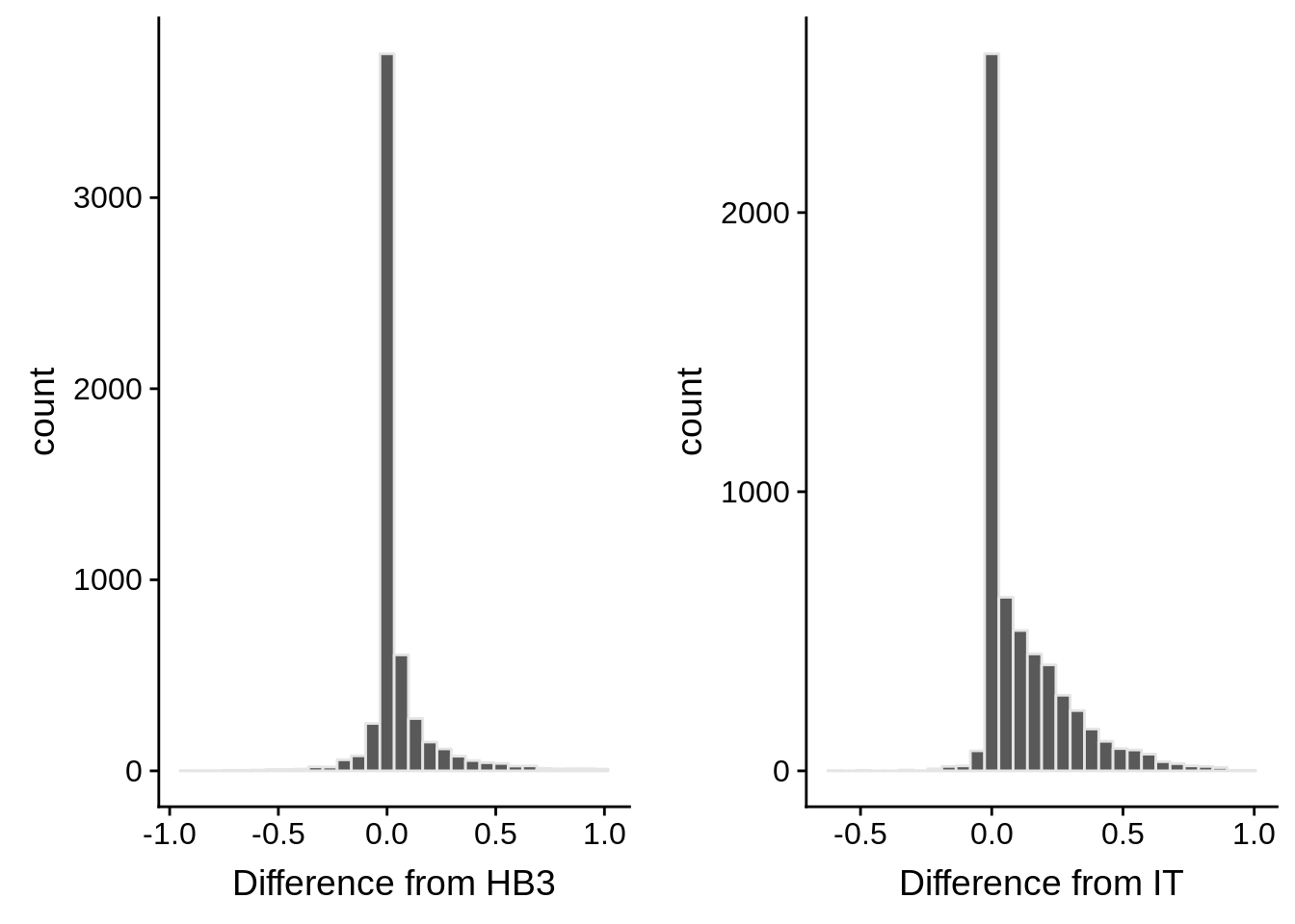
Expand here to see past versions of unnamed-chunk-5-1.png:
| Version | Author | Date |
|---|---|---|
| acf38fa | Philipp Ross | 2018-10-07 |
g <- ggplot(mean_coverages,aes(x=`3D7`,y=HB3)) + geom_point() + geom_point(data=mean_coverages %>% dplyr::filter(gene_id == "PF3D7_1222600"),color = "#E41A1C") + geom_text(data=mean_coverages %>% dplyr::filter(gene_id == "PF3D7_1222600"),label="PF3D7_1222600", color = "#E41A1C", hjust = 1.1)
print(g)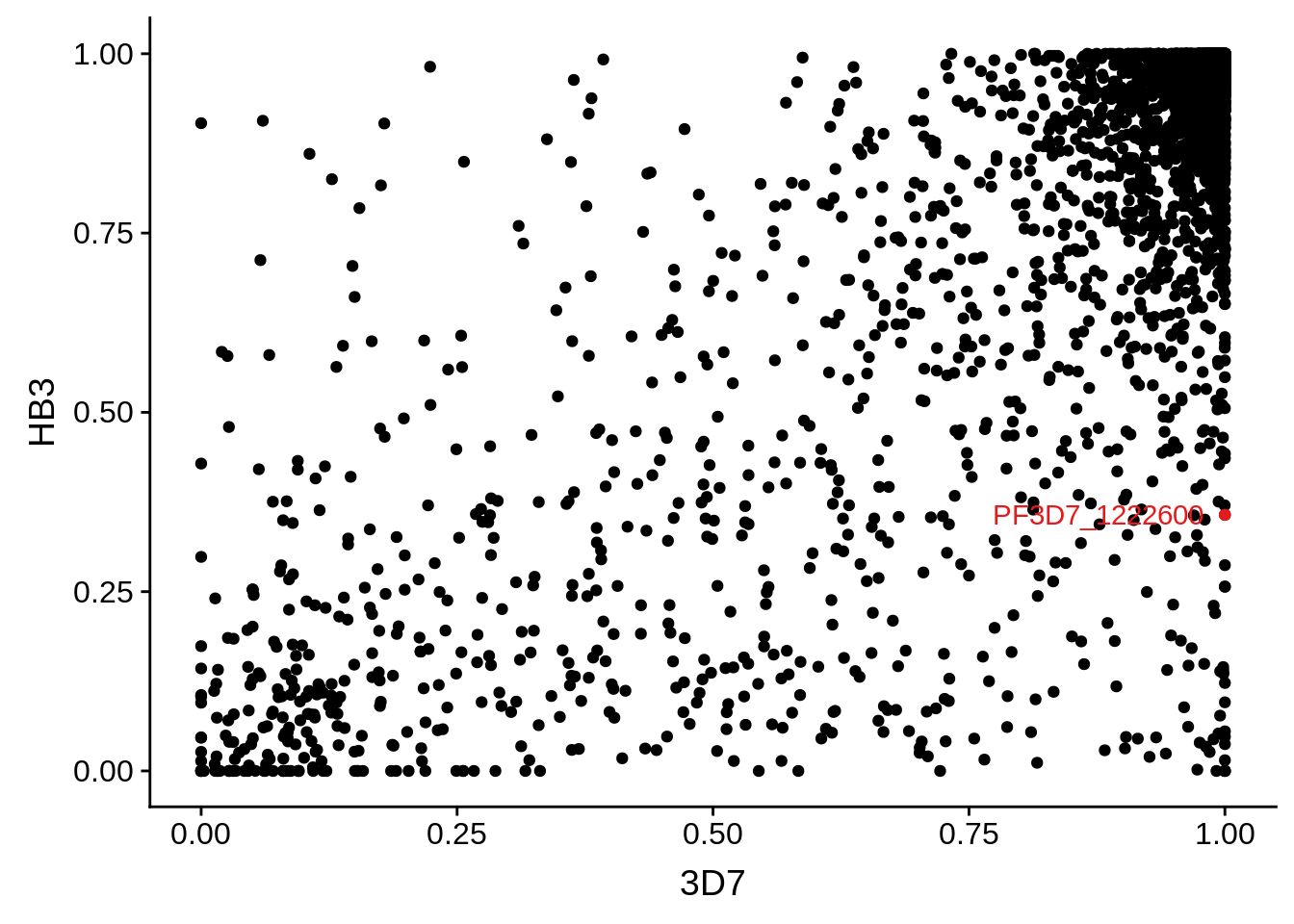
Expand here to see past versions of unnamed-chunk-6-1.png:
| Version | Author | Date |
|---|---|---|
| acf38fa | Philipp Ross | 2018-10-07 |
g <- ggplot(mean_coverages,aes(x=`3D7`,y=HB3)) + geom_point() + geom_point(data=mean_coverages %>% dplyr::filter(gene_id == "PF3D7_0930300"),color = "#E41A1C") + geom_text(data=mean_coverages %>% dplyr::filter(gene_id == "PF3D7_0930300"),label="PF3D7_0930300", color = "#E41A1C", hjust = 1.1)
print(g)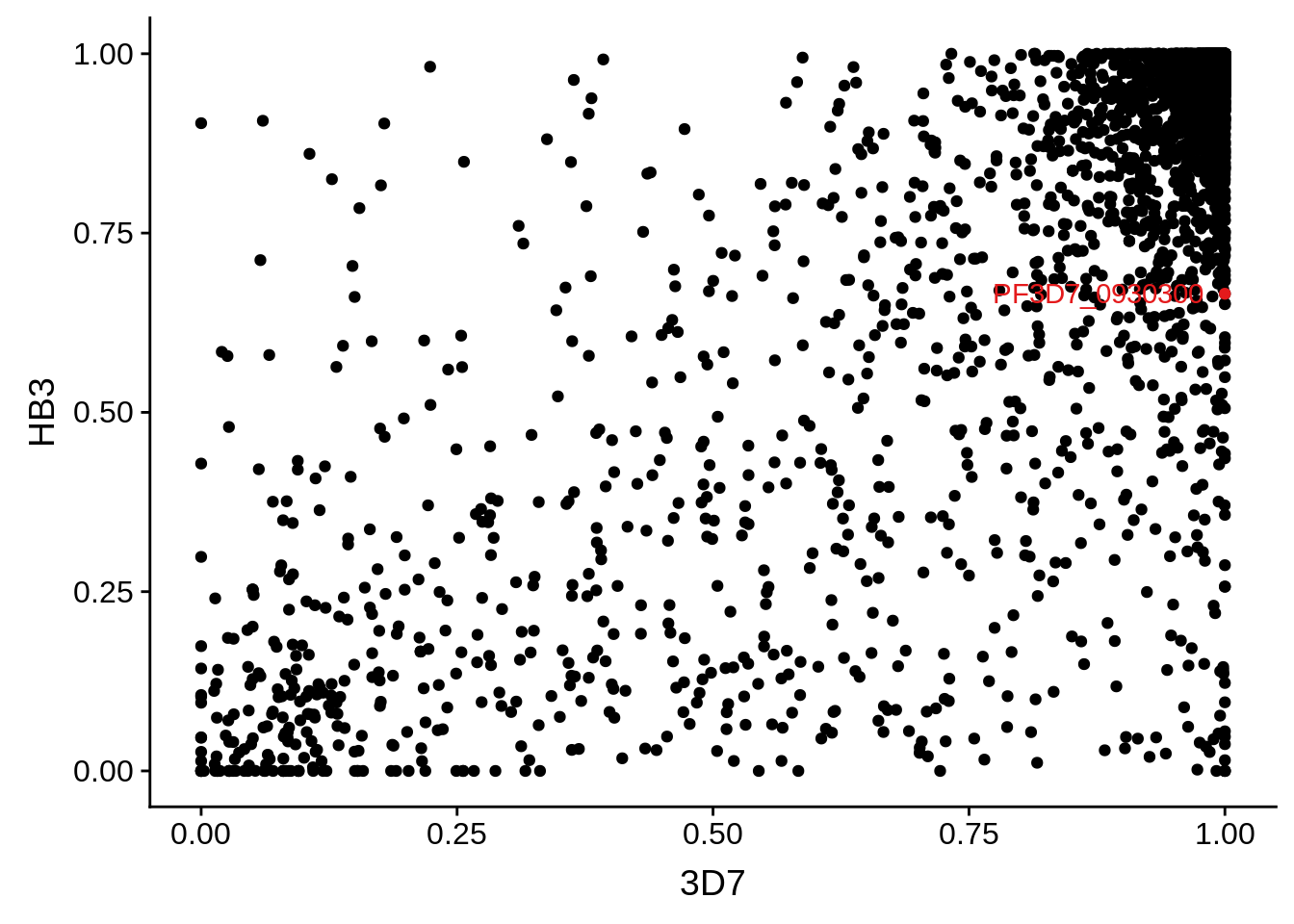
g <- ggplot(mean_coverages,aes(x=`3D7`,y=HB3)) + geom_point() + geom_point(data=mean_coverages %>% dplyr::filter(`3D7`<0.25 & HB3 >0.75),color = "#E41A1C") + geom_text(data=mean_coverages %>% dplyr::filter(`3D7`<0.25 & HB3 >0.75), aes(label=gene_id), color = "#E41A1C", hjust = -0.5, check_overlap = TRUE)
print(g)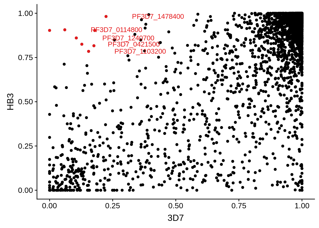
Expand here to see past versions of unnamed-chunk-7-1.png:
| Version | Author | Date |
|---|---|---|
| acf38fa | Philipp Ross | 2018-10-07 |
g <- ggplot(mean_coverages,aes(x=`3D7`,y=IT)) + geom_point() + geom_point(data=mean_coverages %>% dplyr::filter(`3D7`<0.5 & IT >0.5),color = "#E41A1C") + geom_text(data=mean_coverages %>% dplyr::filter(`3D7`<0.5 & IT >0.5), aes(label=gene_id), color = "#E41A1C", hjust = -0.5, check_overlap = TRUE)
print(g)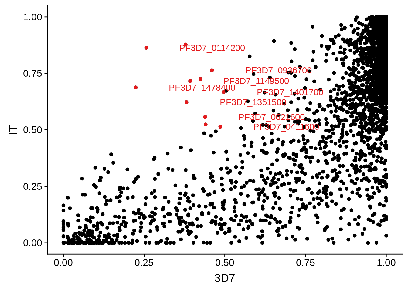
Expand here to see past versions of unnamed-chunk-8-1.png:
| Version | Author | Date |
|---|---|---|
| acf38fa | Philipp Ross | 2018-10-07 |
g <- ggplot(mean_coverages,aes(x=IT,y=HB3)) + geom_point() + geom_point(data=mean_coverages %>% dplyr::filter(IT<0.25 & HB3 >0.75),color = "#E41A1C") + geom_text(data=mean_coverages %>% dplyr::filter(IT<0.25 & HB3 >0.75), aes(label=gene_id), color = "#E41A1C", hjust = -0.5, check_overlap = TRUE)
print(g)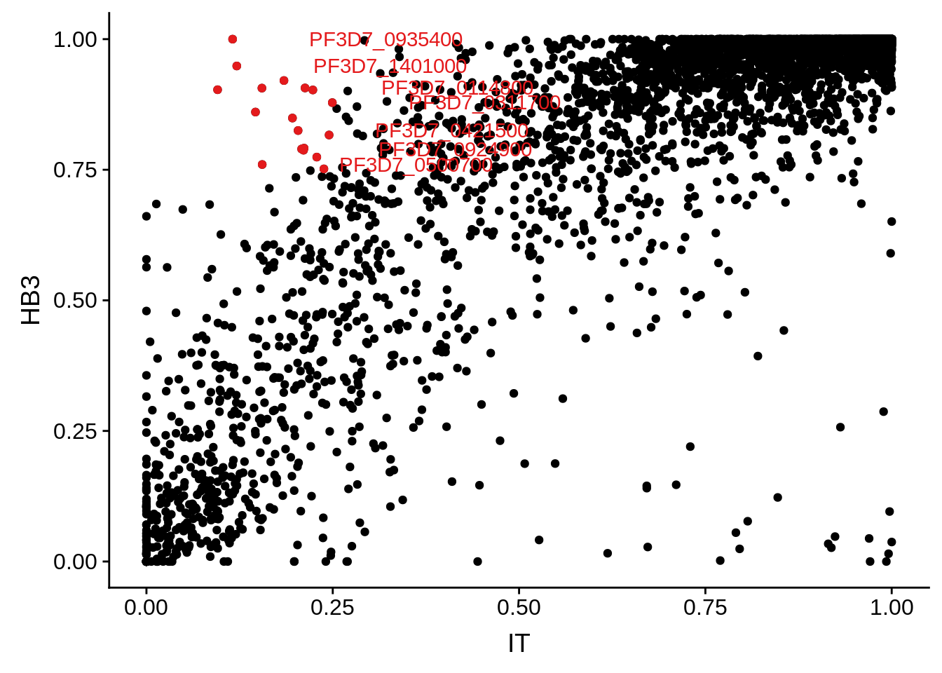
Results
Some genes may barely get over the threshold of 5 TPMs, which was chosen arbitrarily. We are not interested in those results. We want to see what transcripts are clearly abundant in one strain, while clearly absent or at the very least severely down-regulated in another strain. The question then becomes whether this is due to poor coverage across the gene (highly polymorphic) or actual low transcript copy number. MSP1 is an example of a highly polymorphic gene in HB3 versus 3D7. It is not covered very well across the gene and thus has been marked as “undetected.” MSP2 is an example of a gene that is detected, but is also highly polymorphic.
Looking through this CGH data will help as well: http://www.ncbi.nlm.nih.gov/pmc/articles/PMC2901668/
Off in HB3 not in 3D7
Off in 3D7 not in HB3
Off in IT not in 3D7
Off in 3D7 not in IT
Off in IT not in HB3
Session information
R version 3.5.0 (2018-04-23)
Platform: x86_64-pc-linux-gnu (64-bit)
Running under: Gentoo/Linux

Matrix products: default
BLAS: /usr/local/lib64/R/lib/libRblas.so
LAPACK: /usr/local/lib64/R/lib/libRlapack.so

locale:
 [1] LC_CTYPE=en_US.UTF-8       LC_NUMERIC=C
 [3] LC_TIME=en_US.UTF-8        LC_COLLATE=en_US.UTF-8
 [5] LC_MONETARY=en_US.UTF-8    LC_MESSAGES=en_US.UTF-8
 [7] LC_PAPER=en_US.UTF-8       LC_NAME=C
 [9] LC_ADDRESS=C               LC_TELEPHONE=C
[11] LC_MEASUREMENT=en_US.UTF-8 LC_IDENTIFICATION=C

attached base packages:
[1] parallel  stats4    stats     graphics  grDevices utils     datasets
[8] methods   base

other attached packages:
 [1] bindrcpp_0.2.2
 [2] BSgenome.Pfalciparum.PlasmoDB.v24_1.0
 [3] BSgenome_1.48.0
 [4] rtracklayer_1.40.6
 [5] Biostrings_2.48.0
 [6] XVector_0.20.0
 [7] GenomicRanges_1.32.7
 [8] GenomeInfoDb_1.16.0
 [9] org.Pf.plasmo.db_3.6.0
[10] AnnotationDbi_1.42.1
[11] IRanges_2.14.12
[12] S4Vectors_0.18.3
[13] Biobase_2.40.0
[14] BiocGenerics_0.26.0
[15] scales_1.0.0
[16] cowplot_0.9.3
[17] magrittr_1.5
[18] forcats_0.3.0
[19] stringr_1.3.1
[20] dplyr_0.7.6
[21] purrr_0.2.5
[22] readr_1.1.1
[23] tidyr_0.8.1
[24] tibble_1.4.2
[25] ggplot2_3.0.0
[26] tidyverse_1.2.1

loaded via a namespace (and not attached):
 [1] nlme_3.1-137                bitops_1.0-6
 [3] matrixStats_0.54.0          lubridate_1.7.4
 [5] bit64_0.9-7                 httr_1.3.1
 [7] rprojroot_1.3-2             tools_3.5.0
 [9] backports_1.1.2             DT_0.4
[11] R6_2.3.0                    DBI_1.0.0
[13] lazyeval_0.2.1              colorspace_1.3-2
[15] withr_2.1.2                 tidyselect_0.2.4
[17] bit_1.1-14                  compiler_3.5.0
[19] git2r_0.23.0                cli_1.0.1
[21] rvest_0.3.2                 xml2_1.2.0
[23] DelayedArray_0.6.6          labeling_0.3
[25] digest_0.6.17               Rsamtools_1.32.3
[27] rmarkdown_1.10              R.utils_2.7.0
[29] pkgconfig_2.0.2             htmltools_0.3.6
[31] htmlwidgets_1.3             rlang_0.2.2
[33] readxl_1.1.0                rstudioapi_0.8
[35] RSQLite_2.1.1               shiny_1.1.0
[37] bindr_0.1.1                 jsonlite_1.5
[39] crosstalk_1.0.0             BiocParallel_1.14.2
[41] R.oo_1.22.0                 RCurl_1.95-4.11
[43] GenomeInfoDbData_1.1.0      Matrix_1.2-14
[45] Rcpp_0.12.19                munsell_0.5.0
[47] R.methodsS3_1.7.1           stringi_1.2.4
[49] whisker_0.3-2               yaml_2.2.0
[51] SummarizedExperiment_1.10.1 zlibbioc_1.26.0
[53] plyr_1.8.4                  grid_3.5.0
[55] blob_1.1.1                  promises_1.0.1
[57] crayon_1.3.4                lattice_0.20-35
[59] haven_1.1.2                 hms_0.4.2
[61] knitr_1.20                  pillar_1.3.0
[63] XML_3.98-1.16               glue_1.3.0
[65] evaluate_0.11               modelr_0.1.2
[67] httpuv_1.4.5                cellranger_1.1.0
[69] gtable_0.2.0                assertthat_0.2.0
[71] mime_0.5                    xtable_1.8-3
[73] broom_0.5.0                 later_0.7.5
[75] GenomicAlignments_1.16.0    memoise_1.1.0
[77] workflowr_1.1.1
This reproducible R Markdown analysis was created with workflowr 1.1.1