GC bias sanity check
Philipp Ross
2018-09-25
Last updated: 2018-09-25
Code version: fa4fca8
We wanted to see whether the sequencing protocol properly got rid of most GC bias signals. To do this we had to calculate the coverage and GC content across transcript windows and plot them in several different ways.
Methods
Here I describe the methods for looking at GC content bias in the RNA-seq data with and without UTRs. The workflow is the following:
- Create GFF3 formatted files for core, protein-coding genes
- Create a file that includes 5’ and 3’ UTRs for core-protein-coding genes, only
- Break each exon into 50bp windows using bedtools
- Calculate the the nucleotide content using bedtools nuc
- Calculate the coverage over each 50bp window using bedtools multicov
- Merge the counts and nucleotide content file into one and convert counts into RPKMs
- Normalize the RPKMs by the median RPKM across the entire trasnscript; this normalizes the RPKM of the window by the RPKM of the transcript it comes from
- Look at GC bias in various ways:
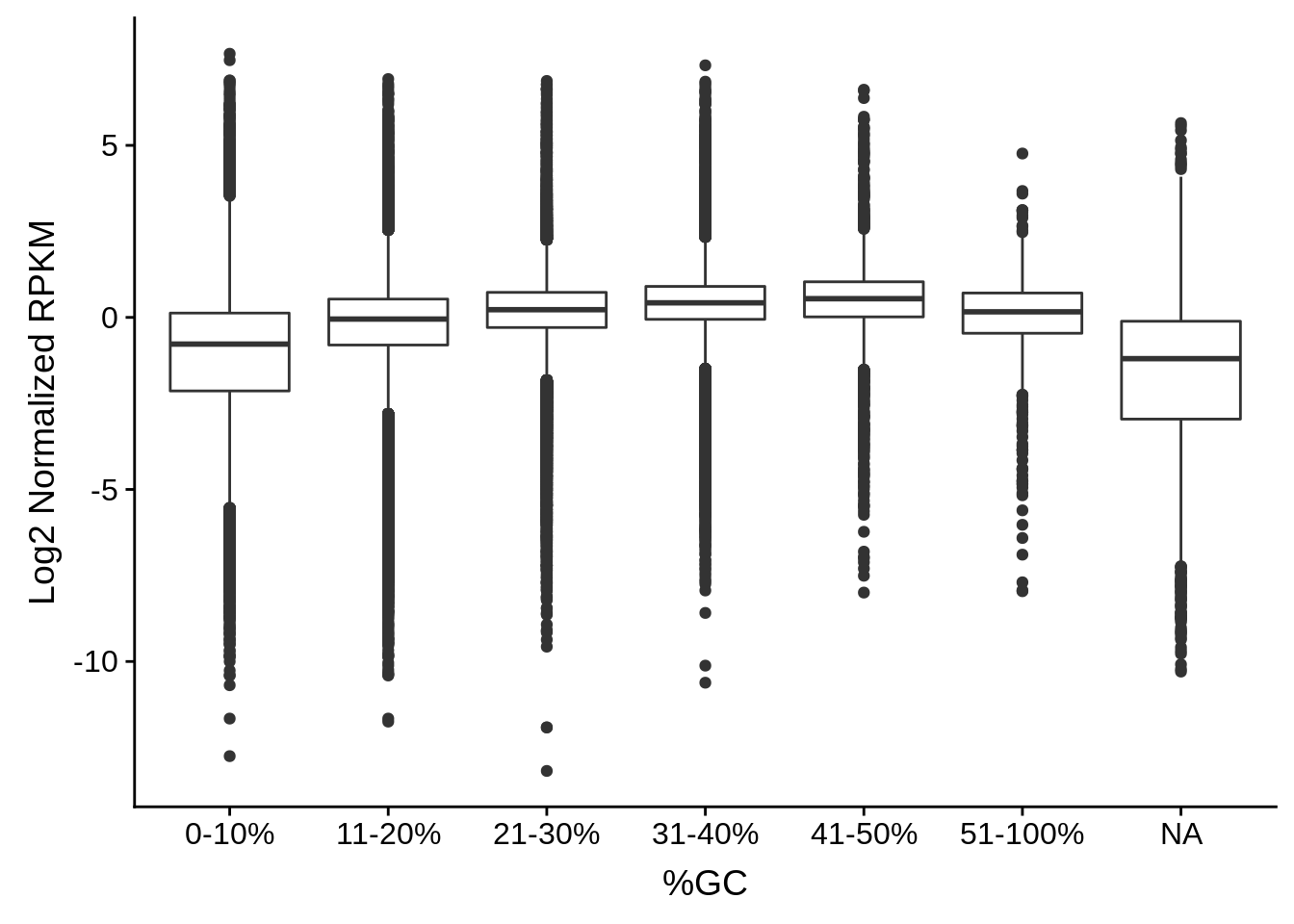
- Bin windows by GC content and consider the average expression of each window over time
- Plot the GC content by normalized RPKM
- Plot the GC content and normalized RPKM across individual transcript positions and bin transcripts by their length
In these plots we only include transcripts expressed at 5 RPKMs or more.
The code is included in the scripts/gcbias folder on github. Here we can just visualize some of the results.
First we write some functions:
# Plot gcbias scatter plots for individual transcripts
plot_gcbias_scatter <- function(df, gene) {

  df %>%
    dplyr::filter(id == gene) %>%
    dplyr::group_by(id, pos) %>%
    dplyr::summarise(gc = unique(gc), exp = mean(exp)) %>%
    ggplot(aes(x=gc,y=exp)) +
    geom_point(alpha=0.75) +
    stat_smooth(color="red",method="lm") +
    ggtitle(gene) +
    ylab("Normalized Expression") +
    xlab("%GC")

}

# Plot gcbias scatter plots for multiple transcripts
plot_gcbias_scatter2 <- function(df) {

  df %>%
    dplyr::group_by(id, pos) %>%
    dplyr::summarise(gc=unique(gc),exp=mean(exp,na.rm=T)) %>%
    dplyr::group_by(pos) %>%
    dplyr::summarise(gc=mean(gc),exp=mean(exp,na.rm=T)) %>%
    ggplot(aes(x=gc,y=exp)) +
    geom_point(alpha=0.75) +
    stat_smooth(color="red",method="lm") +
    ggtitle(paste("Average of",length(unique(df$id)),"transcripts")) +
    ylab("Normalized Expression") +
    xlab("%GC")

}

# Plot gcbias across individual transcripts
plot_gcbias_transcript <- function(df, gene) {

  g1 <- df %>%
    dplyr::filter(id == gene) %>%
    dplyr::group_by(id, pos) %>%
    dplyr::summarise(gc = unique(gc), exp = mean(exp)) %>%
    ggplot(aes(x=pos,y=exp)) +
    stat_smooth(color="blue",se=F,span=0.15) +
    ylab("Normalized Expression") +
    xlab("") +
    ggtitle(gene) +
    theme(axis.text.x = element_blank(),
          axis.ticks.x = element_blank(),
          axis.line.x = element_blank()) +
    geom_hline(yintercept = 1, linetype=2)

  g2 <- df %>%
    dplyr::filter(id == gene) %>%
    dplyr::group_by(id, pos) %>%
    dplyr::summarise(gc = unique(gc), exp = mean(exp)) %>%
    ggplot(aes(x=pos,y=gc)) +
    stat_smooth(color="red",se=F,span=0.15) +
    ylab("%GC") +
    xlab("Position")

  cowplot::plot_grid(g1,g2,nrow=2,align="v", rel_heights = c(2, 1))
}

# Plot gcbias across multiple transcripts
plot_gcbias_transcript2 <- function(df) {

  g1 <- df %>%
    dplyr::group_by(id, pos) %>%
    dplyr::summarise(exp=mean(exp,na.rm=T)) %>%
    dplyr::group_by(pos) %>%
    dplyr::summarise(exp=mean(exp,na.rm=T)) %>%
    ggplot(aes(x=pos,y=exp)) +
    stat_smooth(color="blue",se=F,span=0.25) +
    geom_point(color="blue") +
    ylab("Normalized Expression") +
    xlab("") +
    scale_x_continuous(limits=c(1,max(unique(df$pos)))) +
    ggtitle(paste("Average of",length(unique(df$id)),"transcripts")) +
    geom_hline(yintercept = 1, linetype=2)

  g2 <- df %>%
    dplyr::group_by(id, pos) %>%
    dplyr::summarise(gc=unique(gc)) %>%
    dplyr::group_by(pos) %>%
    dplyr::summarise(gc=mean(gc)) %>%
    ggplot(aes(x=pos,y=gc)) +
    stat_smooth(color="red",se=F,span=0.25) +
    geom_point(color="red") +
    ylab("%GC") +
    xlab("Position") +
    scale_x_continuous(limits=c(1,max(unique(df$pos))))

  cowplot::plot_grid(g1,g2,nrow=2,align="v",rel_heights=c(1, 1))

}

# Plot gcbias across transcripts on top of each other
# Since ggplot2 doesn't let you create two plots using two different
# y-axes I needed to use the basic plot function in R
plot_gcbias_transcript3 <- function(df, gene) {

  if(gene %in% df$id) {

    what <- df %>%
       dplyr::filter(id == gene) %>%
       dplyr::spread(tp,exp)

    what$exp <- apply(what, 1, function(row) {
      mean(c(as.numeric(row[["tp1"]]),
             as.numeric(row[["tp2"]]),
             as.numeric(row[["tp3"]]),
             as.numeric(row[["tp4"]]),
             as.numeric(row[["tp5"]]),
             as.numeric(row[["tp6"]]),
             as.numeric(row[["tp7"]])))
    })

    if(sum(is.na(what$exp)) == 0) {

      par(mar = c(5,5,2,5))
      with(what, plot(pos, predict(loess(exp ~ pos,span=0.25)),
                      type="l",
                      col="blue",
                      ylab="Normalized Expression",
                      xlab="Transcript Position (5' - 3')",
                      lwd=2,
                      main=gene))
      abline(h=1,lty=2,col="grey2")

      par(new = T)
      with(what, plot(pos, predict(loess(gc ~ pos,span=0.25)),
                      type="l",col="red3",axes=F, xlab=NA, ylab=NA,lwd=1,lty=3))
      axis(side=4)
      mtext(side=4,line=3,"%GC")

    }

  } else {
    print(paste(gene, "NA"))
  }

}

# Bin the windows by GC content and plot boxplots of the normalized
# exprssion values within those bins
plot_gcbias_boxplot <- function(df, include) {

  # remove genes if only meant to include certain genes
  if(sum(!is.na(include))>0) {
    df <- df %>%
      filter(id %in% include)
  }

  df$bins <- as.character(cut(df$gc, breaks=c(0,0.1,0.2,0.3,0.4,0.5,1.0),
        labels=c("0-10%","11-20%","21-30%","31-40%","41-50%","51-100%")))

  df %>%
    dplyr::select(-gc) %>%
    dplyr::group_by(id, pos) %>%
    dplyr::summarise(exp = mean(exp), bins = dplyr::first(bins)) %>%
    ggplot(aes(x=bins,y=log2(exp))) +
    geom_boxplot() +
    xlab("%GC") +
    ylab("Log2 Normalized RPKM")
}
And now we plot the data.
3D7
include <- readr::read_tsv("../data/gcbias/on3d7.txt",col_names=F)$X1
bias_file <- readRDS("../data/gcbias/3d7_core_cds_exons_with_utrs_50bp_windows.rds")

# get transcripts we care about
tmp25 <- bias_file %>%
  group_by(id) %>%
  summarise(m = max(pos)) %>%
  filter(m < 25) %$%
  id

tmp50 <- bias_file %>%
  group_by(id) %>%
  summarise(m = max(pos)) %>%
  filter(m >= 25 & m <= 50) %$%
  id

tmp75 <- bias_file %>%
  group_by(id) %>%
  summarise(m = max(pos)) %>%
  filter(m >= 50 & m <= 75) %$%
  id

tmp100 <- bias_file %>%
  group_by(id) %>%
  summarise(m = max(pos)) %>%
  filter(m >= 75 & m <= 100) %$%
  id

tmpgt <- bias_file %>%
  group_by(id) %>%
  summarise(m = max(pos)) %>%
  filter(m > 100) %$%
  id

# some transcripts overlap...can't get position. Don't include these
ugh <- bias_file %>%
  group_by(id, pos) %>%
  summarise(l = length(unique(gc))) %>%
  filter(l > 1) %$%
  unique(id)

# plot gcbias as a scatter plot
g <- bias_file %>% filter(id %in% tmp25 & id %in% include & !(id %in% ugh)) %>% plot_gcbias_scatter2()
print(g)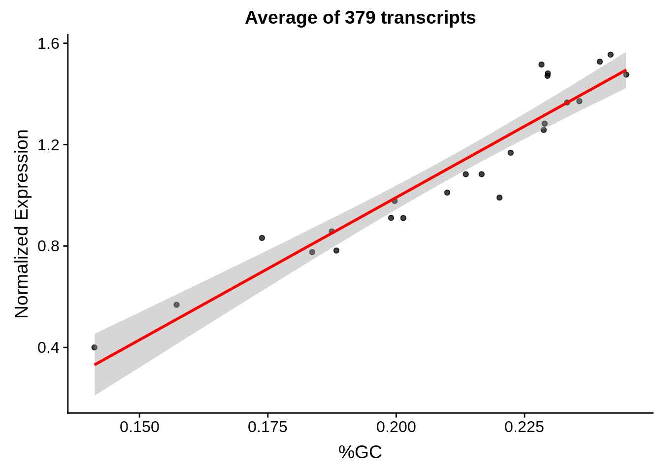
g <- bias_file %>% filter(id %in% tmp50 & id %in% include & !(id %in% ugh)) %>% plot_gcbias_scatter2()
print(g)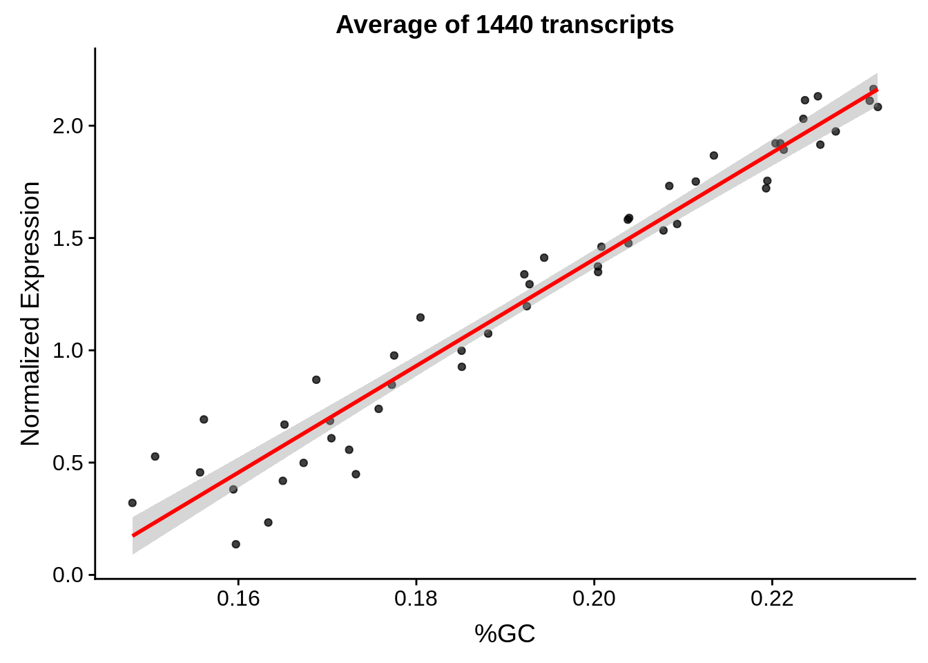
g <- bias_file %>% filter(id %in% tmp75 & id %in% include & !(id %in% ugh)) %>% plot_gcbias_scatter2()
print(g)
g <- bias_file %>% filter(id %in% tmp100 & id %in% include & !(id %in% ugh)) %>% plot_gcbias_scatter2()
print(g)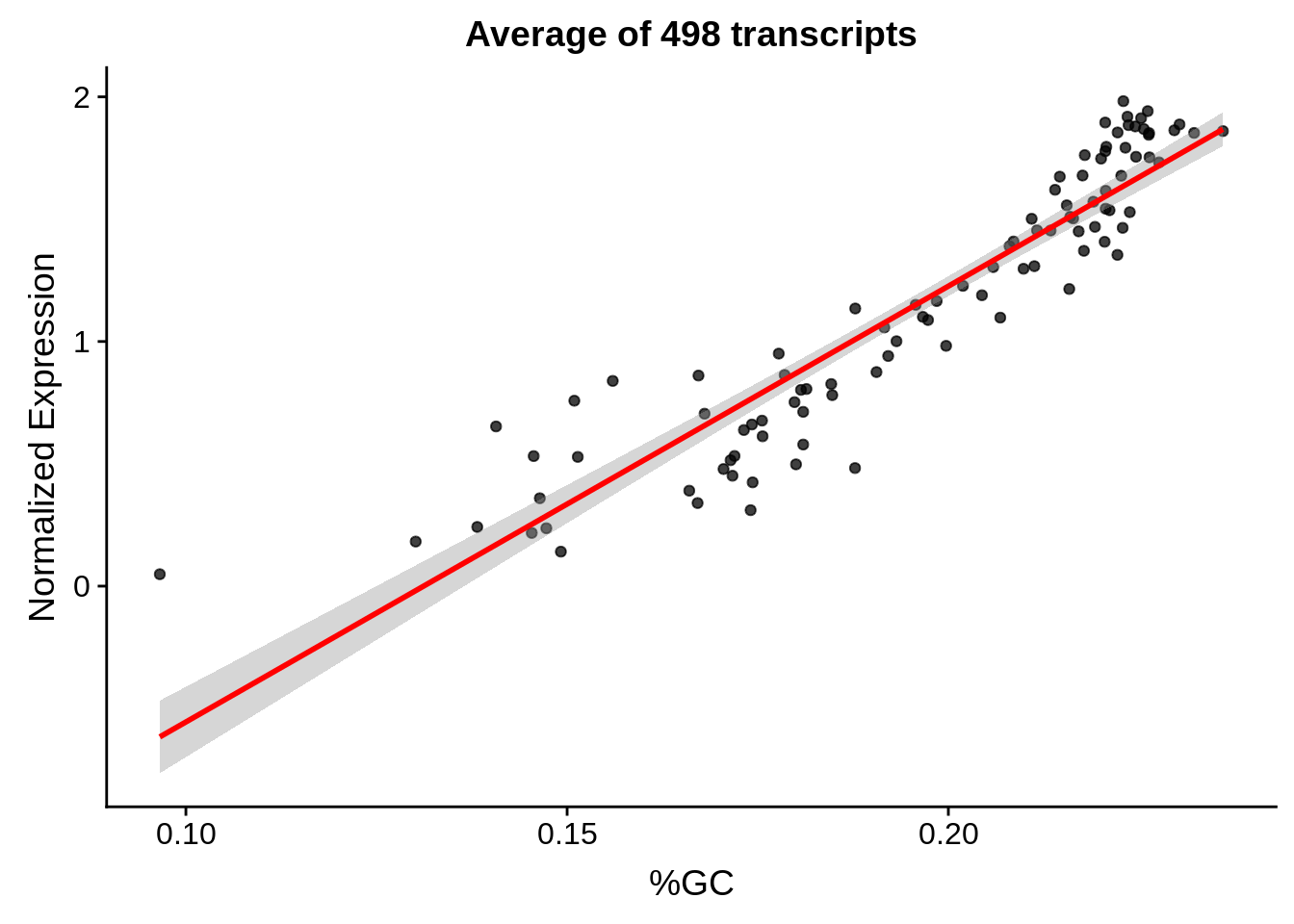
g <- bias_file %>% filter(id %in% tmpgt & id %in% include & !(id %in% ugh)) %>% plot_gcbias_scatter2()
print(g)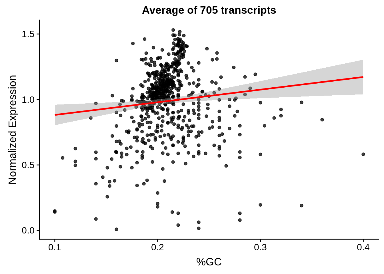
# plot gcbias across transcript position
g <- bias_file %>% filter(id %in% tmp25 & id %in% include & !(id %in% ugh)) %>% plot_gcbias_transcript2()
print(g)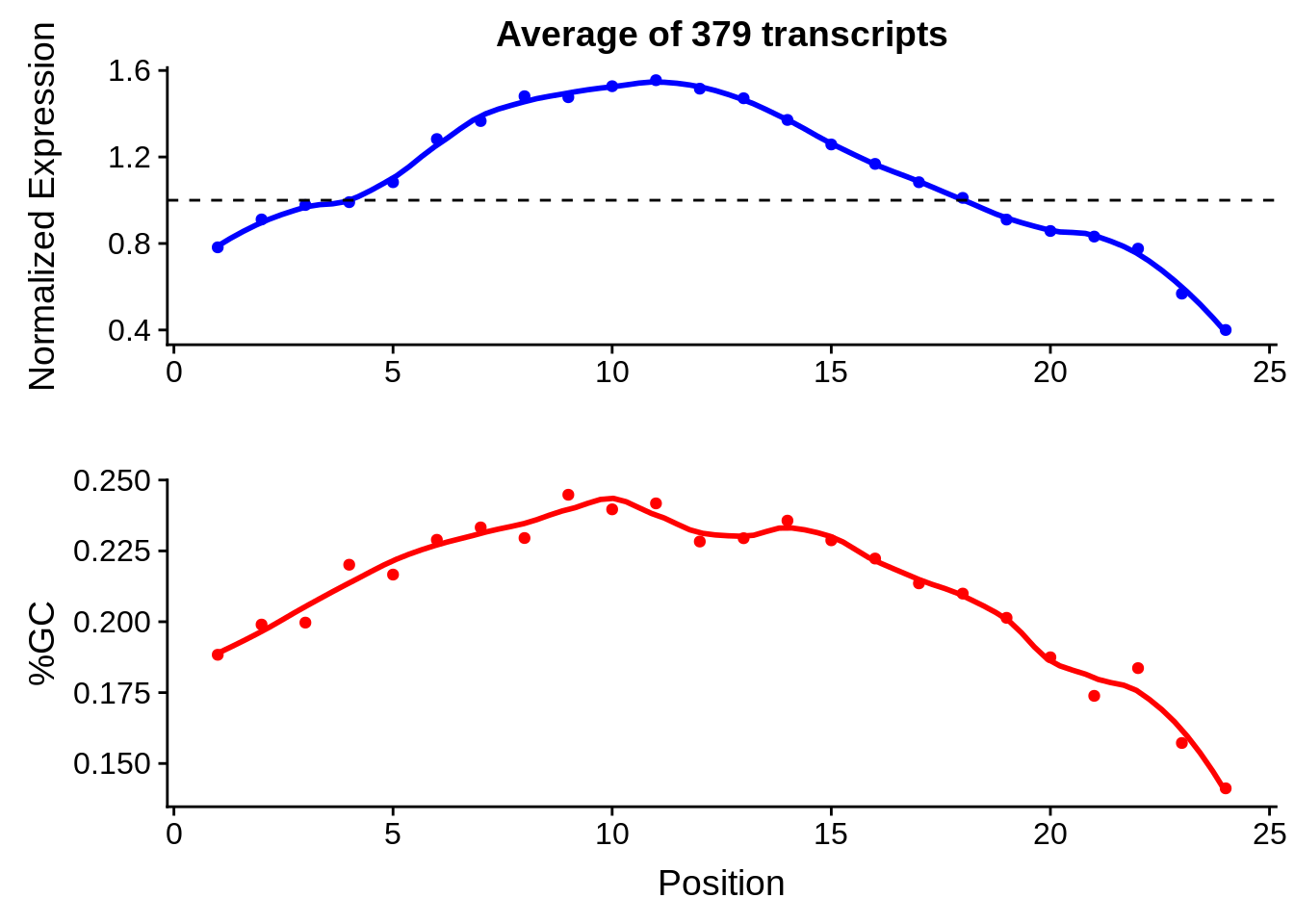
g <- bias_file %>% filter(id %in% tmp50 & id %in% include & !(id %in% ugh)) %>% plot_gcbias_transcript2()
print(g)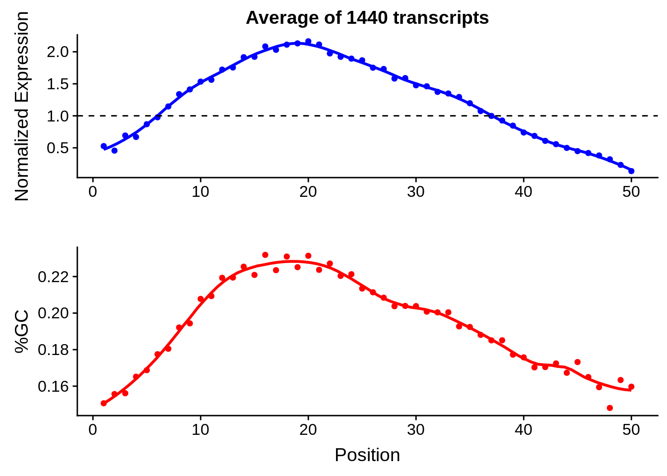
g <- bias_file %>% filter(id %in% tmp75 & id %in% include & !(id %in% ugh)) %>% plot_gcbias_transcript2()
print(g)
g <- bias_file %>% filter(id %in% tmp100 & id %in% include & !(id %in% ugh)) %>% plot_gcbias_transcript2()
print(g)
g <- bias_file %>% filter(id %in% tmpgt & id %in% include & !(id %in% ugh)) %>% plot_gcbias_transcript2()
print(g)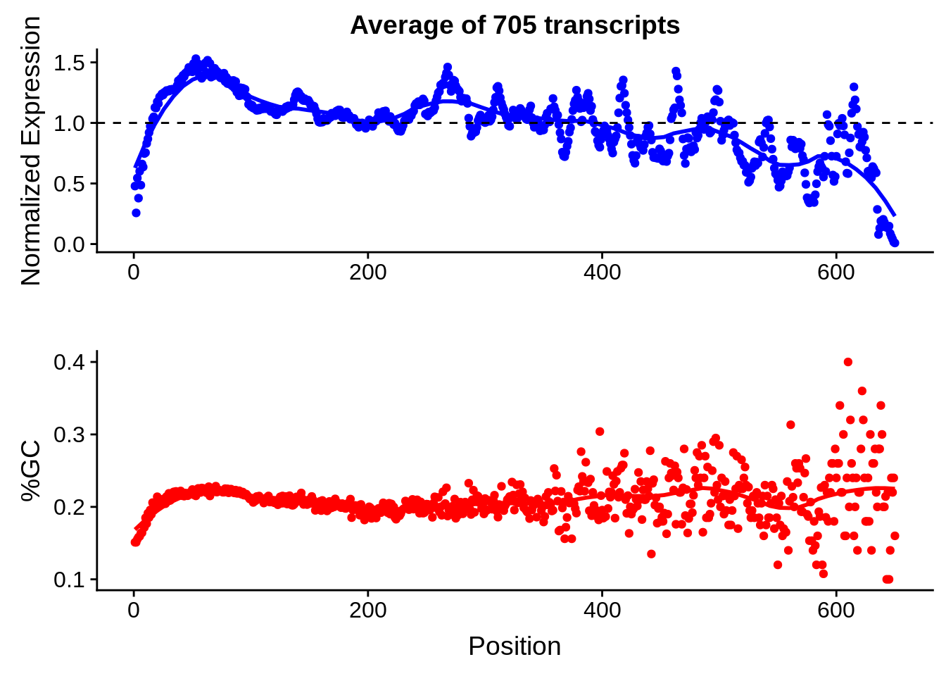

HB3
include <- readr::read_tsv("../data/gcbias/onhb3.txt",col_names=F)$X1
biasfile <- readRDS("../data/gcbias/hb3_core_cds_exons_50bp_windows.rds")

# get transcripts we care about
tmp25 <- bias_file %>%
  group_by(id) %>%
  summarise(m = max(pos)) %>%
  filter(m < 25) %$%
  id

tmp50 <- bias_file %>%
  group_by(id) %>%
  summarise(m = max(pos)) %>%
  filter(m >= 25 & m <= 50) %$%
  id

tmp75 <- bias_file %>%
  group_by(id) %>%
  summarise(m = max(pos)) %>%
  filter(m >= 50 & m <= 75) %$%
  id

tmp100 <- bias_file %>%
  group_by(id) %>%
  summarise(m = max(pos)) %>%
  filter(m >= 75 & m <= 100) %$%
  id

tmpgt <- bias_file %>%
  group_by(id) %>%
  summarise(m = max(pos)) %>%
  filter(m > 100) %$%
  id

# some transcripts overlap...can't get position. Don't include these
ugh <- bias_file %>%
  group_by(id, pos) %>%
  summarise(l = length(unique(gc))) %>%
  filter(l > 1) %$%
  unique(id)

# plot gcbias as a scatter plot
g <- bias_file %>% filter(id %in% tmp25 & id %in% include & !(id %in% ugh)) %>% plot_gcbias_scatter2()
print(g)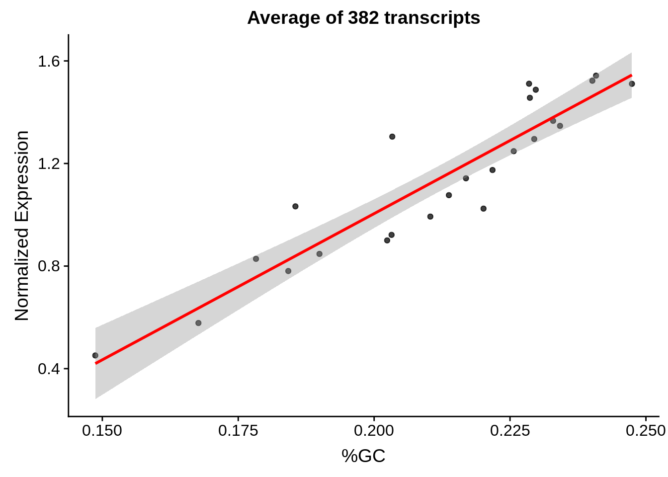
g <- bias_file %>% filter(id %in% tmp50 & id %in% include & !(id %in% ugh)) %>% plot_gcbias_scatter2()
print(g)
g <- bias_file %>% filter(id %in% tmp75 & id %in% include & !(id %in% ugh)) %>% plot_gcbias_scatter2()
print(g)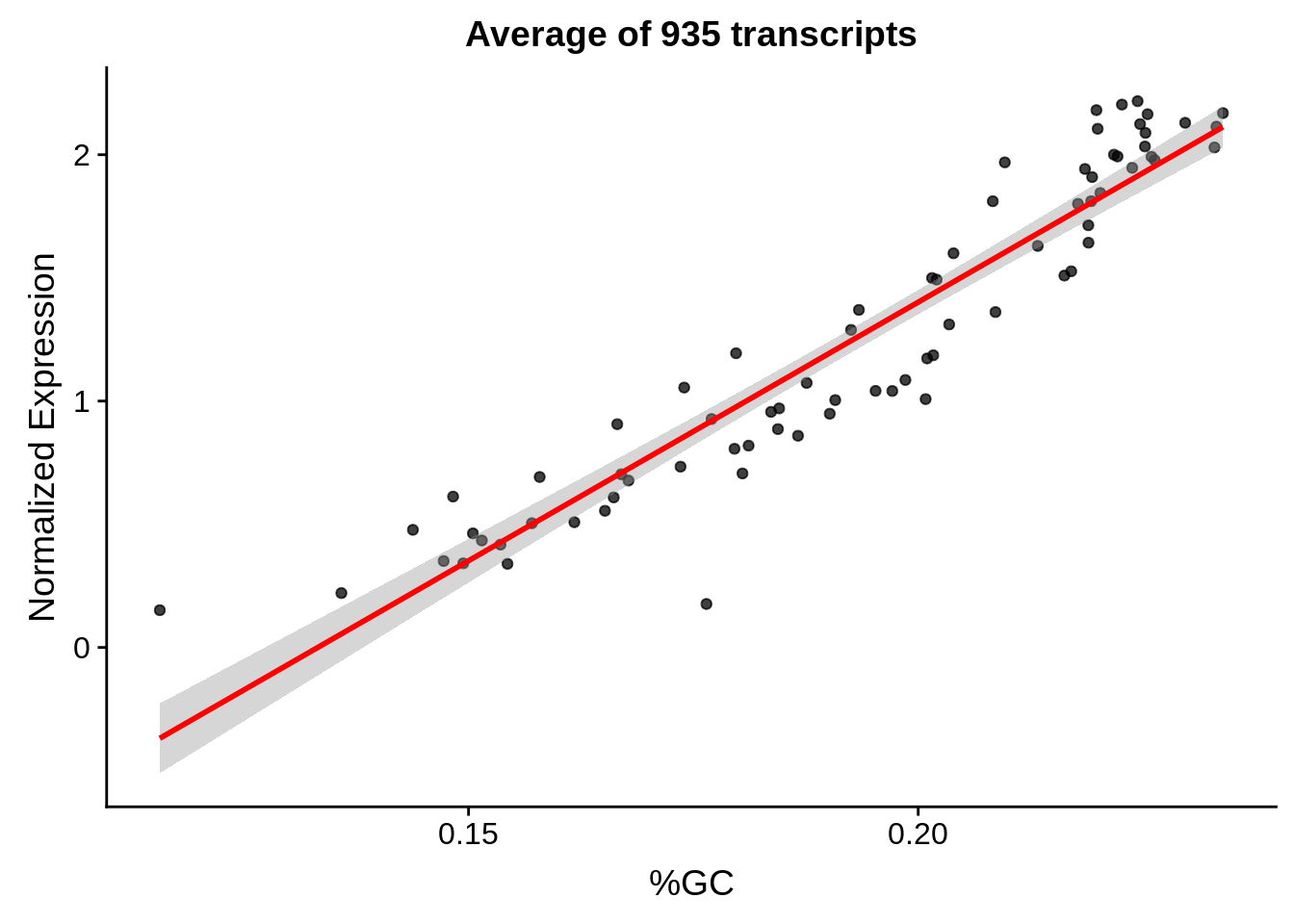
g <- bias_file %>% filter(id %in% tmp100 & id %in% include & !(id %in% ugh)) %>% plot_gcbias_scatter2()
print(g)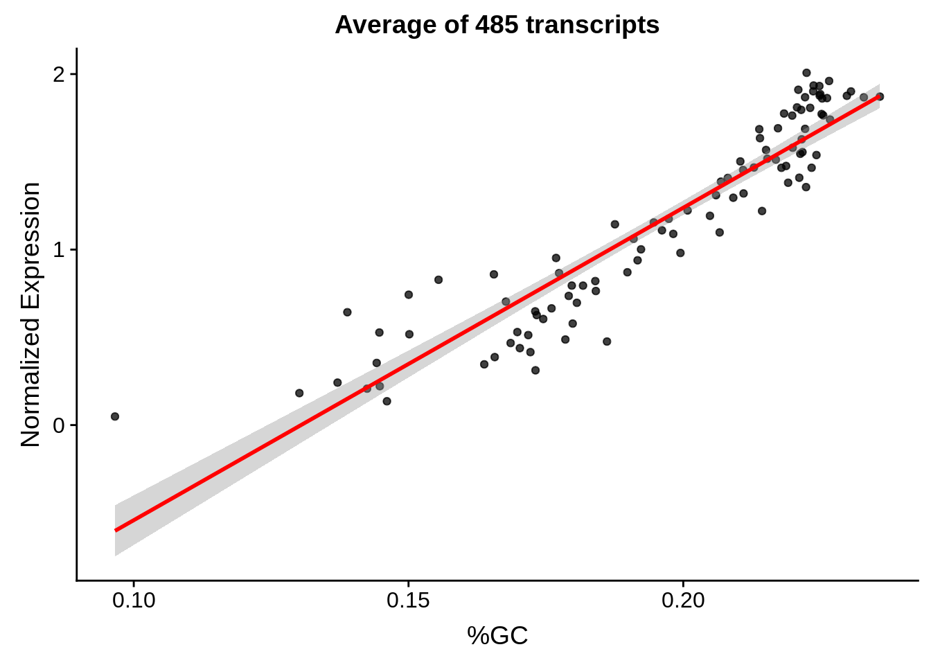
g <- bias_file %>% filter(id %in% tmpgt & id %in% include & !(id %in% ugh)) %>% plot_gcbias_scatter2()
print(g)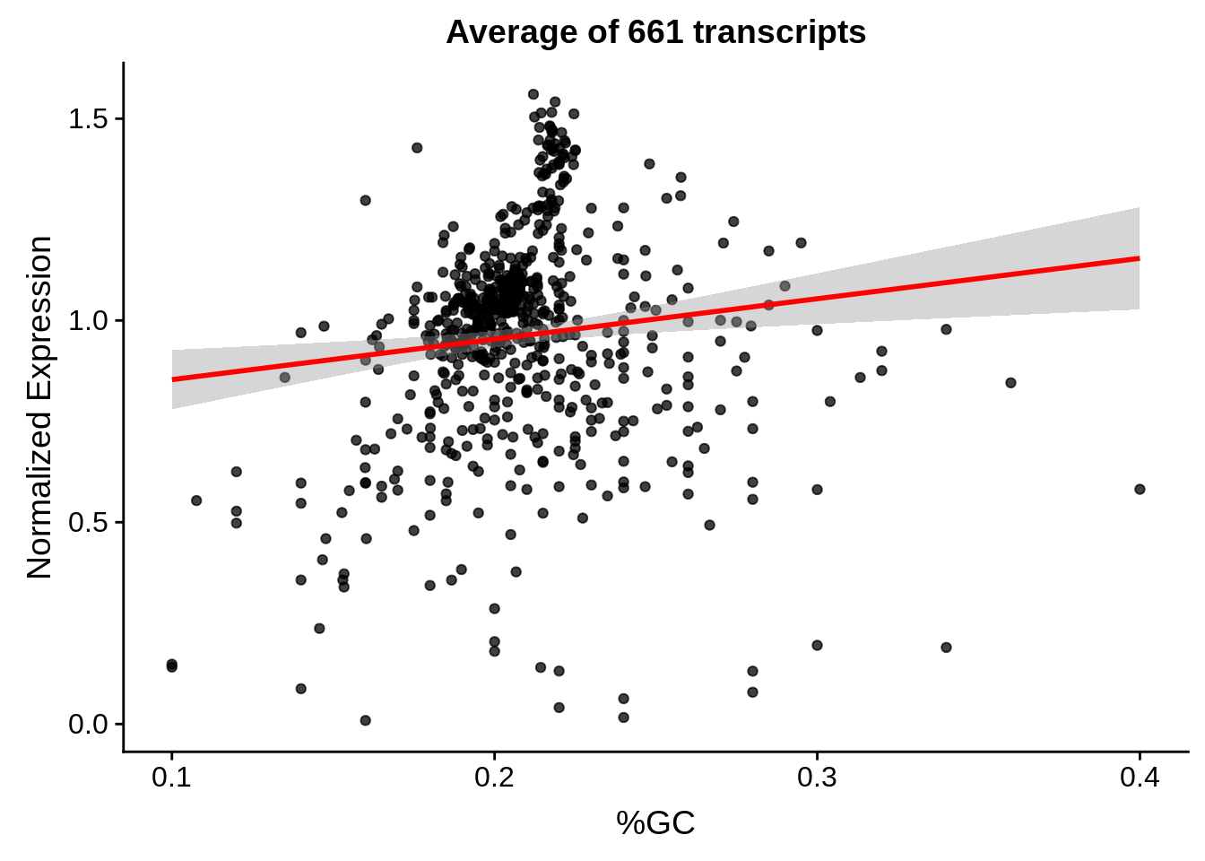
# plot gcbias across transcript position
g <- bias_file %>% filter(id %in% tmp25 & id %in% include & !(id %in% ugh)) %>% plot_gcbias_transcript2()
print(g)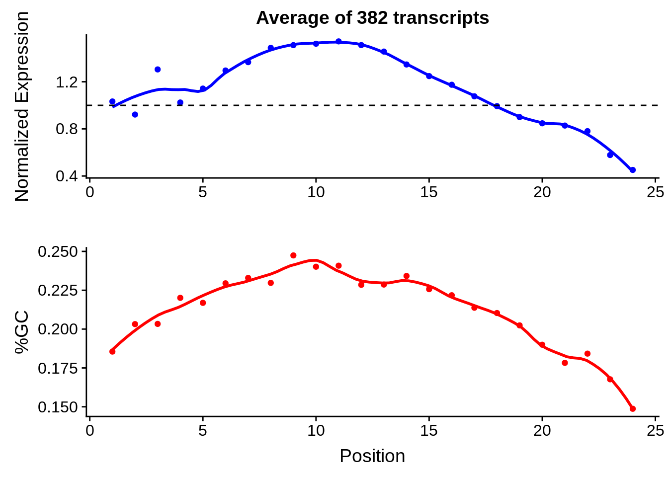
g <- bias_file %>% filter(id %in% tmp50 & id %in% include & !(id %in% ugh)) %>% plot_gcbias_transcript2()
print(g)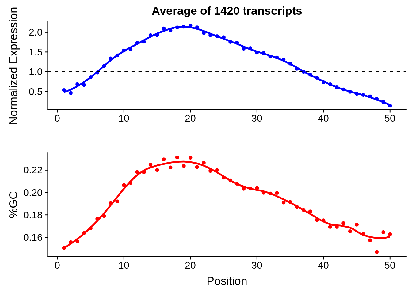
g <- bias_file %>% filter(id %in% tmp75 & id %in% include & !(id %in% ugh)) %>% plot_gcbias_transcript2()
print(g)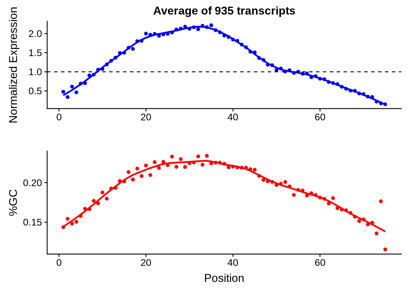
g <- bias_file %>% filter(id %in% tmp100 & id %in% include & !(id %in% ugh)) %>% plot_gcbias_transcript2()
print(g)
g <- bias_file %>% filter(id %in% tmpgt & id %in% include & !(id %in% ugh)) %>% plot_gcbias_transcript2()
print(g)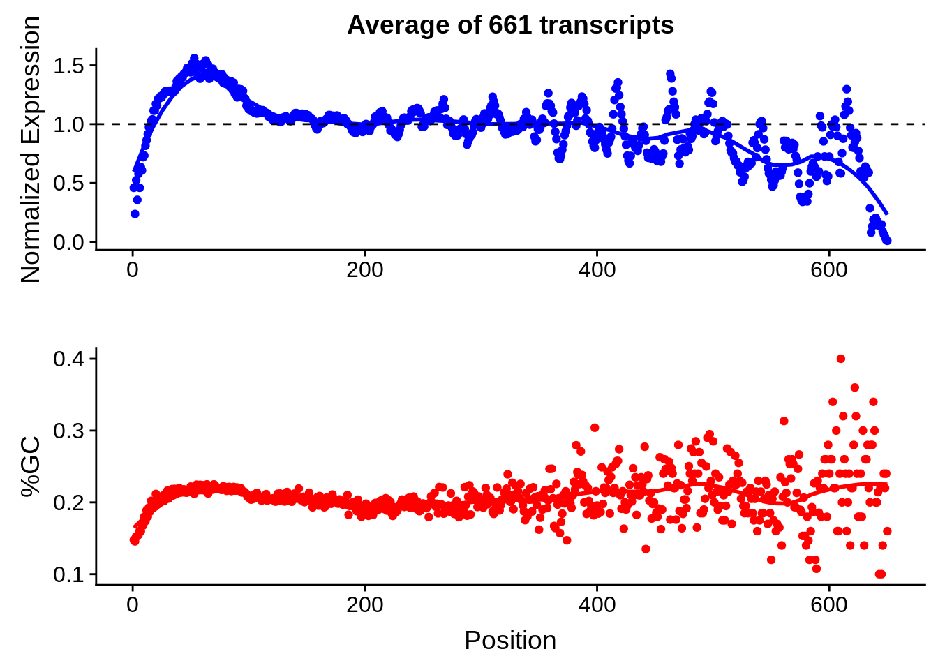
IT
include <- readr::read_tsv("../data/gcbias/onit.txt",col_names=F)$X1
biasfile <- readRDS("../data/gcbias/it_core_cds_exons_50bp_windows.rds")

# get transcripts we care about
tmp25 <- bias_file %>%
  group_by(id) %>%
  summarise(m = max(pos)) %>%
  filter(m < 25) %$%
  id

tmp50 <- bias_file %>%
  group_by(id) %>%
  summarise(m = max(pos)) %>%
  filter(m >= 25 & m <= 50) %$%
  id

tmp75 <- bias_file %>%
  group_by(id) %>%
  summarise(m = max(pos)) %>%
  filter(m >= 50 & m <= 75) %$%
  id

tmp100 <- bias_file %>%
  group_by(id) %>%
  summarise(m = max(pos)) %>%
  filter(m >= 75 & m <= 100) %$%
  id

tmpgt <- bias_file %>%
  group_by(id) %>%
  summarise(m = max(pos)) %>%
  filter(m > 100) %$%
  id

# some transcripts overlap...can't get position. Don't include these
ugh <- bias_file %>%
  group_by(id, pos) %>%
  summarise(l = length(unique(gc))) %>%
  filter(l > 1) %$%
  unique(id)

# plot gcbias as a scatter plot
g <- bias_file %>% filter(id %in% tmp25 & id %in% include & !(id %in% ugh)) %>% plot_gcbias_scatter2()
print(g)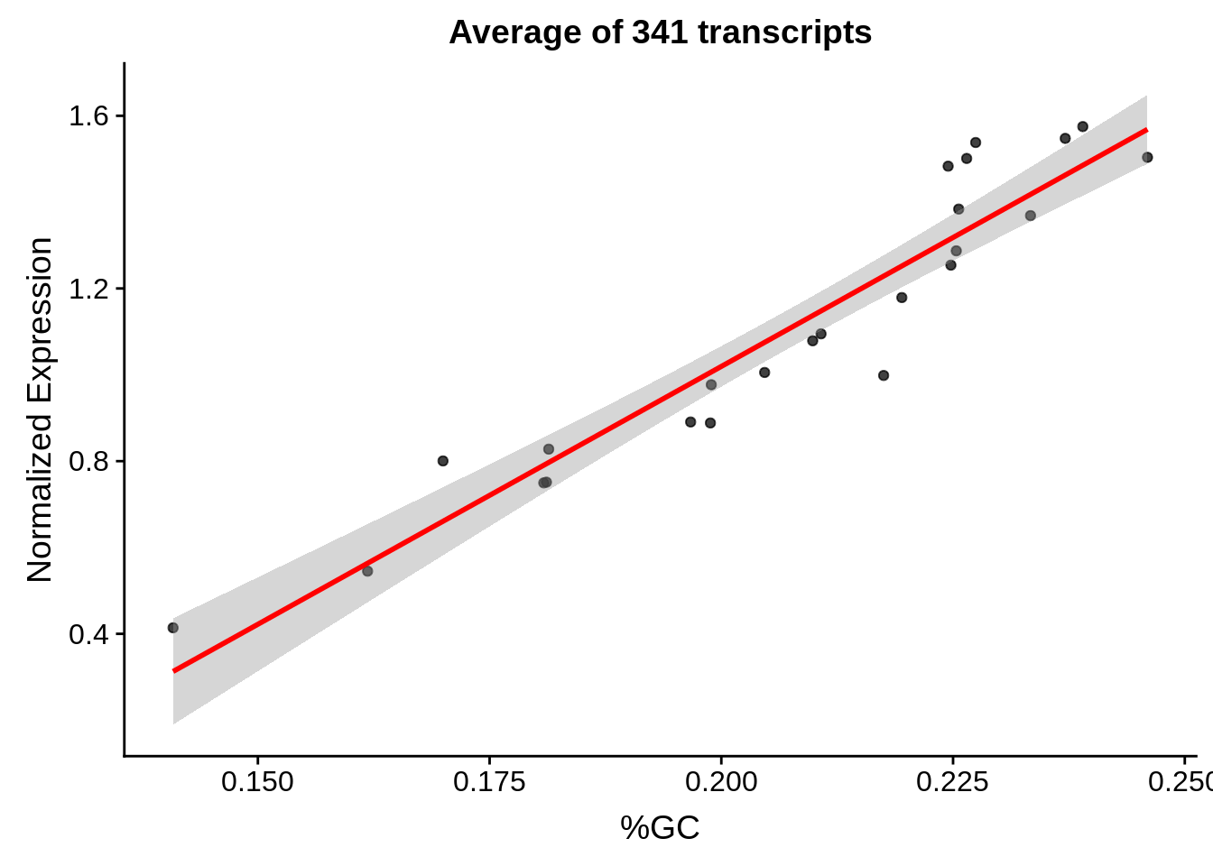
g <- bias_file %>% filter(id %in% tmp50 & id %in% include & !(id %in% ugh)) %>% plot_gcbias_scatter2()
print(g)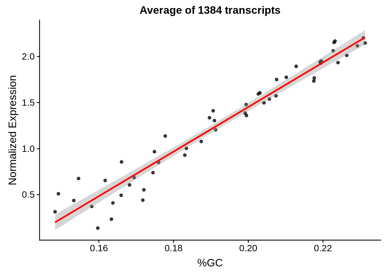
g <- bias_file %>% filter(id %in% tmp75 & id %in% include & !(id %in% ugh)) %>% plot_gcbias_scatter2()
print(g)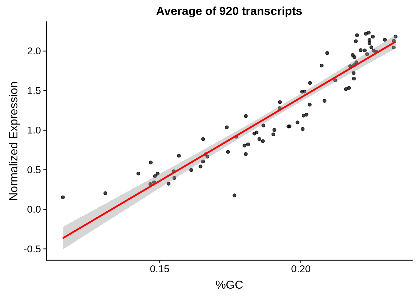
g <- bias_file %>% filter(id %in% tmp100 & id %in% include & !(id %in% ugh)) %>% plot_gcbias_scatter2()
print(g)
g <- bias_file %>% filter(id %in% tmpgt & id %in% include & !(id %in% ugh)) %>% plot_gcbias_scatter2()
print(g)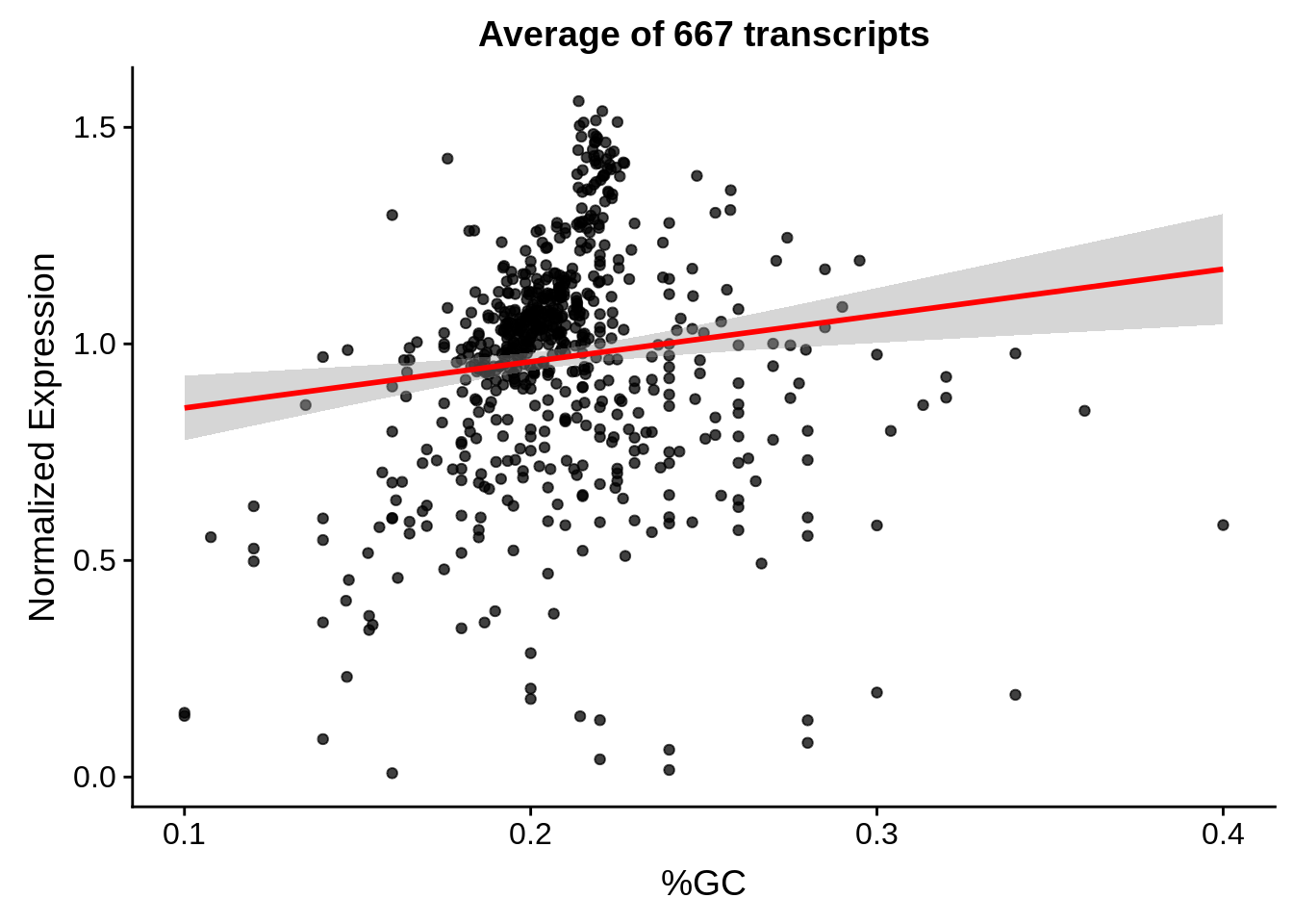
# plot gcbias across transcript position
g <- bias_file %>% filter(id %in% tmp25 & id %in% include & !(id %in% ugh)) %>% plot_gcbias_transcript2()
print(g)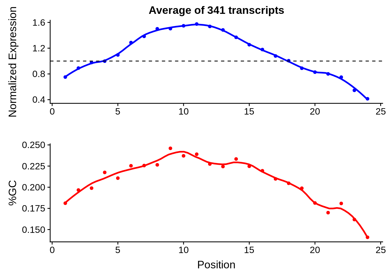
g <- bias_file %>% filter(id %in% tmp50 & id %in% include & !(id %in% ugh)) %>% plot_gcbias_transcript2()
print(g)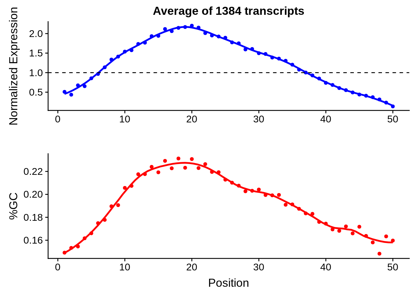
g <- bias_file %>% filter(id %in% tmp75 & id %in% include & !(id %in% ugh)) %>% plot_gcbias_transcript2()
print(g)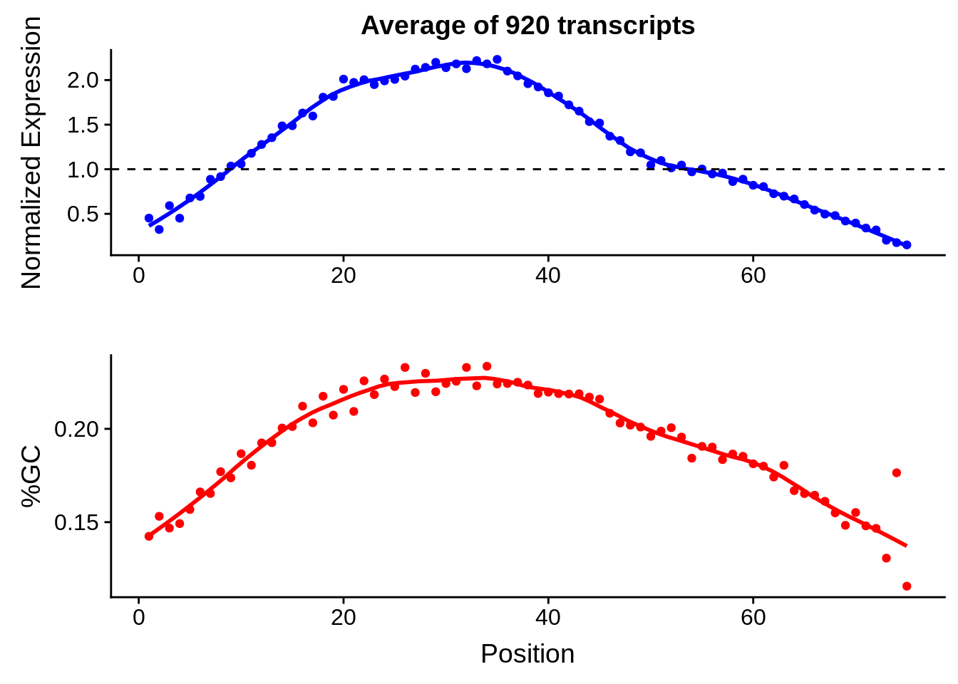
g <- bias_file %>% filter(id %in% tmp100 & id %in% include & !(id %in% ugh)) %>% plot_gcbias_transcript2()
print(g)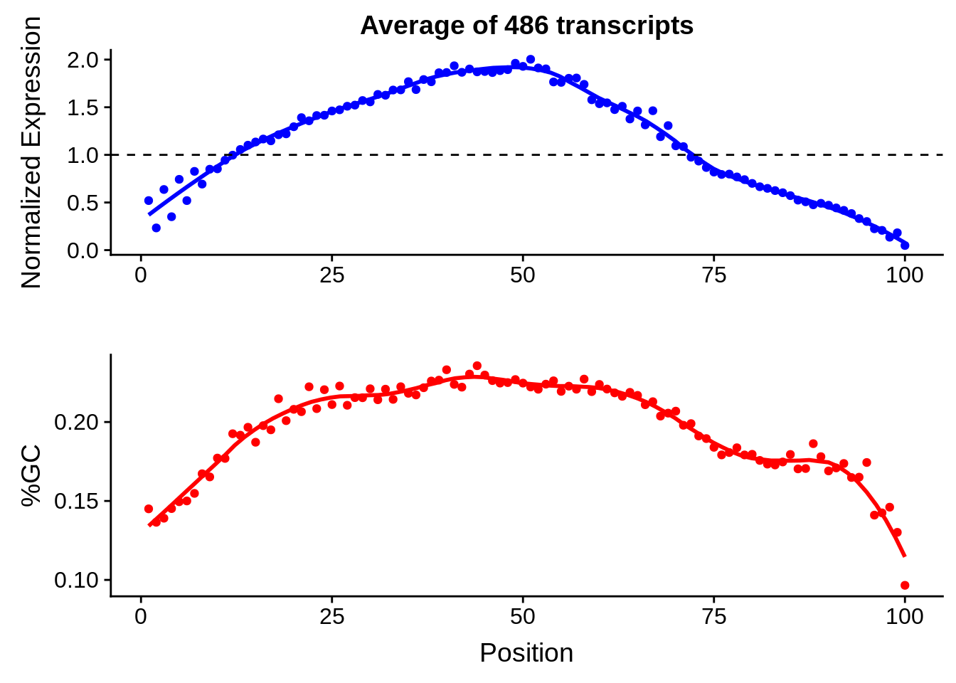
g <- bias_file %>% filter(id %in% tmpgt & id %in% include & !(id %in% ugh)) %>% plot_gcbias_transcript2()
print(g)

Session Information
R version 3.5.0 (2018-04-23)
Platform: x86_64-pc-linux-gnu (64-bit)
Running under: Gentoo/Linux

Matrix products: default
BLAS: /usr/local/lib64/R/lib/libRblas.so
LAPACK: /usr/local/lib64/R/lib/libRlapack.so

locale:
 [1] LC_CTYPE=en_US.UTF-8       LC_NUMERIC=C
 [3] LC_TIME=en_US.UTF-8        LC_COLLATE=en_US.UTF-8
 [5] LC_MONETARY=en_US.UTF-8    LC_MESSAGES=en_US.UTF-8
 [7] LC_PAPER=en_US.UTF-8       LC_NAME=C
 [9] LC_ADDRESS=C               LC_TELEPHONE=C
[11] LC_MEASUREMENT=en_US.UTF-8 LC_IDENTIFICATION=C

attached base packages:
[1] parallel  stats4    stats     graphics  grDevices utils     datasets
[8] methods   base

other attached packages:
 [1] bindrcpp_0.2.2
 [2] BSgenome.Pfalciparum.PlasmoDB.v24_1.0
 [3] BSgenome_1.48.0
 [4] rtracklayer_1.40.6
 [5] Biostrings_2.48.0
 [6] XVector_0.20.0
 [7] GenomicRanges_1.32.6
 [8] GenomeInfoDb_1.16.0
 [9] org.Pf.plasmo.db_3.6.0
[10] AnnotationDbi_1.42.1
[11] IRanges_2.14.10
[12] S4Vectors_0.18.3
[13] Biobase_2.40.0
[14] BiocGenerics_0.26.0
[15] scales_1.0.0
[16] cowplot_0.9.3
[17] magrittr_1.5
[18] forcats_0.3.0
[19] stringr_1.3.1
[20] dplyr_0.7.6
[21] purrr_0.2.5
[22] readr_1.1.1
[23] tidyr_0.8.1
[24] tibble_1.4.2
[25] ggplot2_3.0.0
[26] tidyverse_1.2.1

loaded via a namespace (and not attached):
 [1] nlme_3.1-137                bitops_1.0-6
 [3] matrixStats_0.54.0          lubridate_1.7.4
 [5] bit64_0.9-7                 httr_1.3.1
 [7] rprojroot_1.3-2             tools_3.5.0
 [9] backports_1.1.2             R6_2.2.2
[11] DBI_1.0.0                   lazyeval_0.2.1
[13] colorspace_1.3-2            withr_2.1.2
[15] tidyselect_0.2.4            bit_1.1-14
[17] compiler_3.5.0              git2r_0.23.0
[19] cli_1.0.0                   rvest_0.3.2
[21] xml2_1.2.0                  DelayedArray_0.6.5
[23] labeling_0.3                digest_0.6.15
[25] Rsamtools_1.32.3            rmarkdown_1.10
[27] R.utils_2.6.0               pkgconfig_2.0.2
[29] htmltools_0.3.6             rlang_0.2.2
[31] readxl_1.1.0                rstudioapi_0.7
[33] RSQLite_2.1.1               bindr_0.1.1
[35] jsonlite_1.5                BiocParallel_1.14.2
[37] R.oo_1.22.0                 RCurl_1.95-4.11
[39] GenomeInfoDbData_1.1.0      Matrix_1.2-14
[41] Rcpp_0.12.18                munsell_0.5.0
[43] R.methodsS3_1.7.1           stringi_1.2.4
[45] yaml_2.2.0                  SummarizedExperiment_1.10.1
[47] zlibbioc_1.26.0             plyr_1.8.4
[49] grid_3.5.0                  blob_1.1.1
[51] crayon_1.3.4                lattice_0.20-35
[53] haven_1.1.2                 hms_0.4.2
[55] knitr_1.20                  pillar_1.3.0
[57] XML_3.98-1.16               glue_1.3.0
[59] evaluate_0.11               modelr_0.1.2
[61] cellranger_1.1.0            gtable_0.2.0
[63] assertthat_0.2.0            broom_0.5.0
[65] GenomicAlignments_1.16.0    memoise_1.1.0
[67] workflowr_1.1.1
This R Markdown site was created with workflowr