CTSS clustering

Last updated: 2017-04-10

Code version: 0e2e80a

Generate CTSS files

First thing we need to do is convert the BAM files to CTSS files for CAGEr. Running the following command on each BAM files and combining the stranded files into one individual file will get you the CTSS files:

bedtools genomecov -dz -strand "+" \
  -ibam data/bam/modified_tso/sorted.modified_1nt.sorted.modified.fateseq_3d7_tp1.both.mod.all.out.bam | \
  awk '{print $1,$2,"+",$3}' > out_plus.ctss

bedtools genomecov -dz -strand "-" \
  -ibam data/bam/modified_tso/sorted.modified_1nt.sorted.modified.fateseq_3d7_tp1.both.mod.all.out.bam | \
  awk '{print $1,$2,"-",$3}' > out_minus.ctss
  
cat out_plus.ctss out_minus.ctss | sort -k1,1 -2,2n > out.ctss

Run CAGEr

Now we can run CAGEr on the CTSS files to cluster the tag counts into tag clusters (TCs) and promoter clusters (PCs). The TCs can be thought of as TSSs while the PCs can be thought of as promoter regions with varying architectures.

Rscript code/ctss_clustering run_cager.R data/bam/modified_tso output/ctss_clustering/modified

Exploratory analysis

How many tag clusters do we see and where do we see them?

First we’ll import the tag clusters:

for (tp in seq(1,7)) {
  # generate the file name
  f <- paste0("../output/ctss_clustering/modified/tc",tp,".gff")
  # assign the in read file to a variable
  assign(x = paste0("tc",tp),
         value = rtracklayer::import.gff(f)
         )
  # group by chromosome and count the number of TCs
  dplyr::group_by(tibble::as_tibble(eval(parse(text=paste0("tc",tp)))),seqnames) %>% 
    summarise(n=n())
}
rm(f)

Next we’ll import data on exons, introns, and genes and calculate the proportion of TCs that overlap:

exons.bed    <- rtracklayer::import.bed("../data/annotations/exons_nuclear_3D7_v24.bed") %>%
  tibble::as_tibble() %>%
  dplyr::mutate(anno_name=name,anno_start=start,anno_end=end) %>%
  GenomicRanges::GRanges()
genes.bed    <- rtracklayer::import.bed("../data/annotations/genes_nuclear_3D7_v24.bed")%>%
  tibble::as_tibble() %>%
  dplyr::mutate(anno_name=name,anno_start=start,anno_end=end) %>%
  GenomicRanges::GRanges()
introns.bed  <- rtracklayer::import.bed("../data/annotations/introns_nuclear_3D7_v24.bed")%>%
  tibble::as_tibble() %>%
  dplyr::mutate(anno_name=name,anno_start=start,anno_end=end) %>%
  GenomicRanges::GRanges()

for (tp in seq(1,7)) {
  sum(GenomicRanges::countOverlaps(
    eval(parse(text=paste0("tc",tp))), genes.bed) > 0) / length(eval(parse(text=paste0("tc",tp))))
  sum(GenomicRanges::countOverlaps(
    eval(parse(text=paste0("tc",tp))), exons.bed) > 0) / length(eval(parse(text=paste0("tc",tp))))
  sum(GenomicRanges::countOverlaps(
    eval(parse(text=paste0("tc",tp))), introns.bed) > 0) / length(eval(parse(text=paste0("tc",tp))))
}

What is the size distribution of the tag clusters?

CAGEr creates it’s own plots for this, but we can plot them here as well and do a little more analysis. Let’s import the interquartile widths:

for (tp in seq(1,7)) {
  s <- as_tibble(eval(parse(text=paste0("tc",tp)))) %>% 
    filter(tpm>=2) %$% 
    summary(width)
  print(s)
  g <- as_tibble(eval(parse(text=paste0("tc",tp)))) %>%
    filter(tpm>=2) %>%
    ggplot(aes(x=width)) +
    geom_histogram(color="grey70") +
    ggtitle(paste0("TC",tp))
  print(g)
}

   Min. 1st Qu.  Median    Mean 3rd Qu.    Max. 
   2.00    5.00   12.00   15.87   19.00  310.00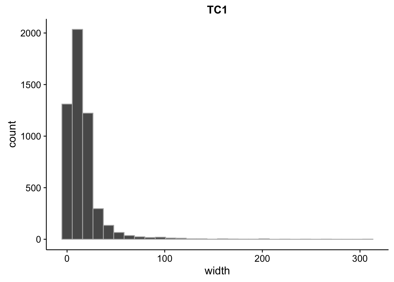

   Min. 1st Qu.  Median    Mean 3rd Qu.    Max. 
   2.00    4.00   10.00   14.33   18.00  257.00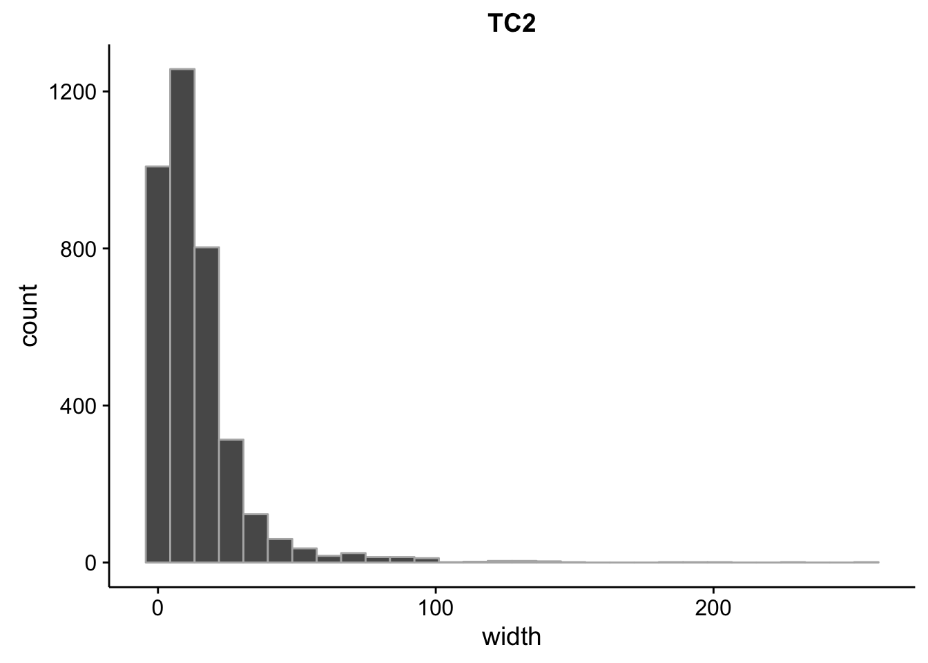

   Min. 1st Qu.  Median    Mean 3rd Qu.    Max. 
   2.00    6.00   13.00   16.55   20.00  256.00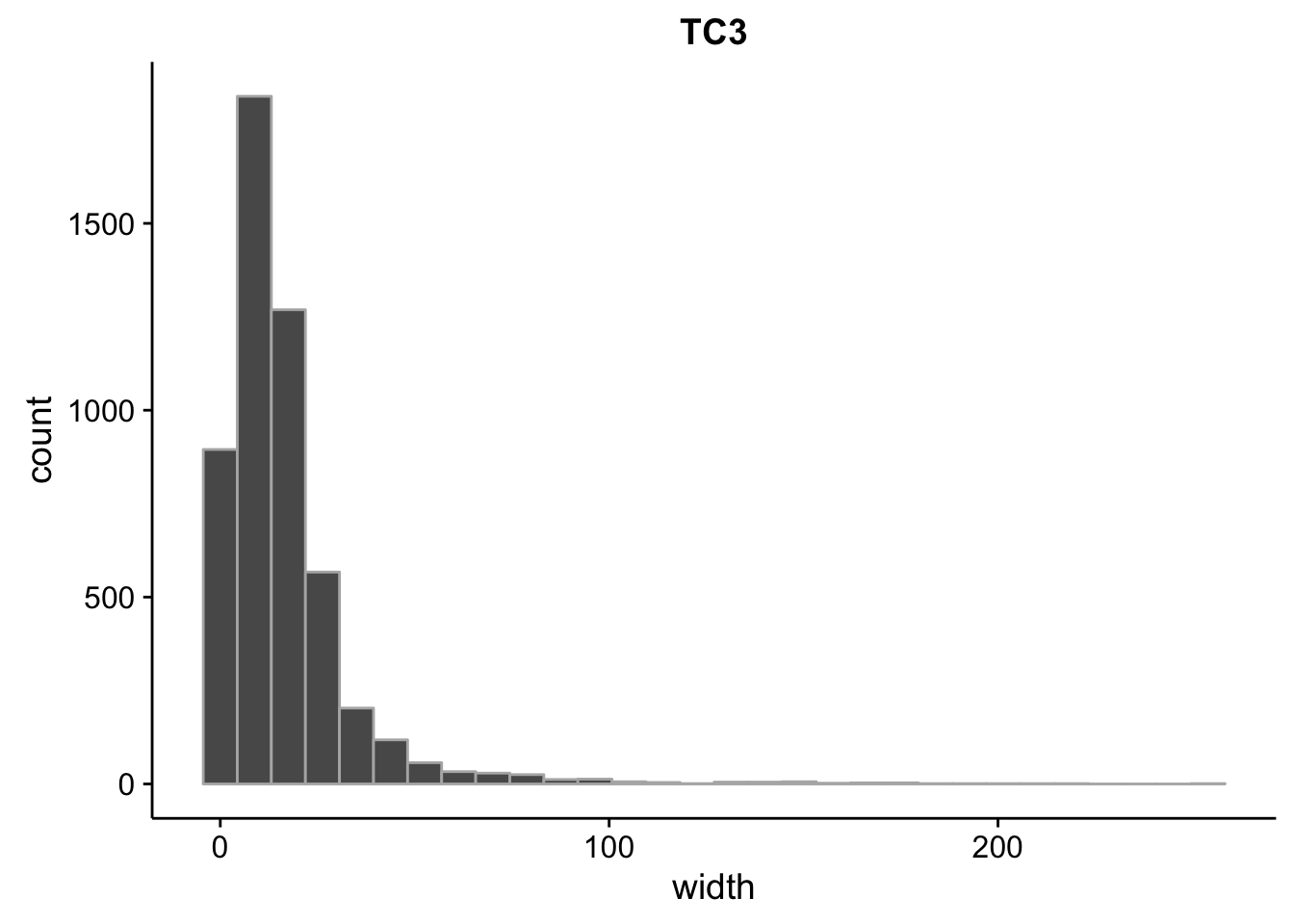

   Min. 1st Qu.  Median    Mean 3rd Qu.    Max. 
   2.00    5.00   12.00   16.85   21.00  240.00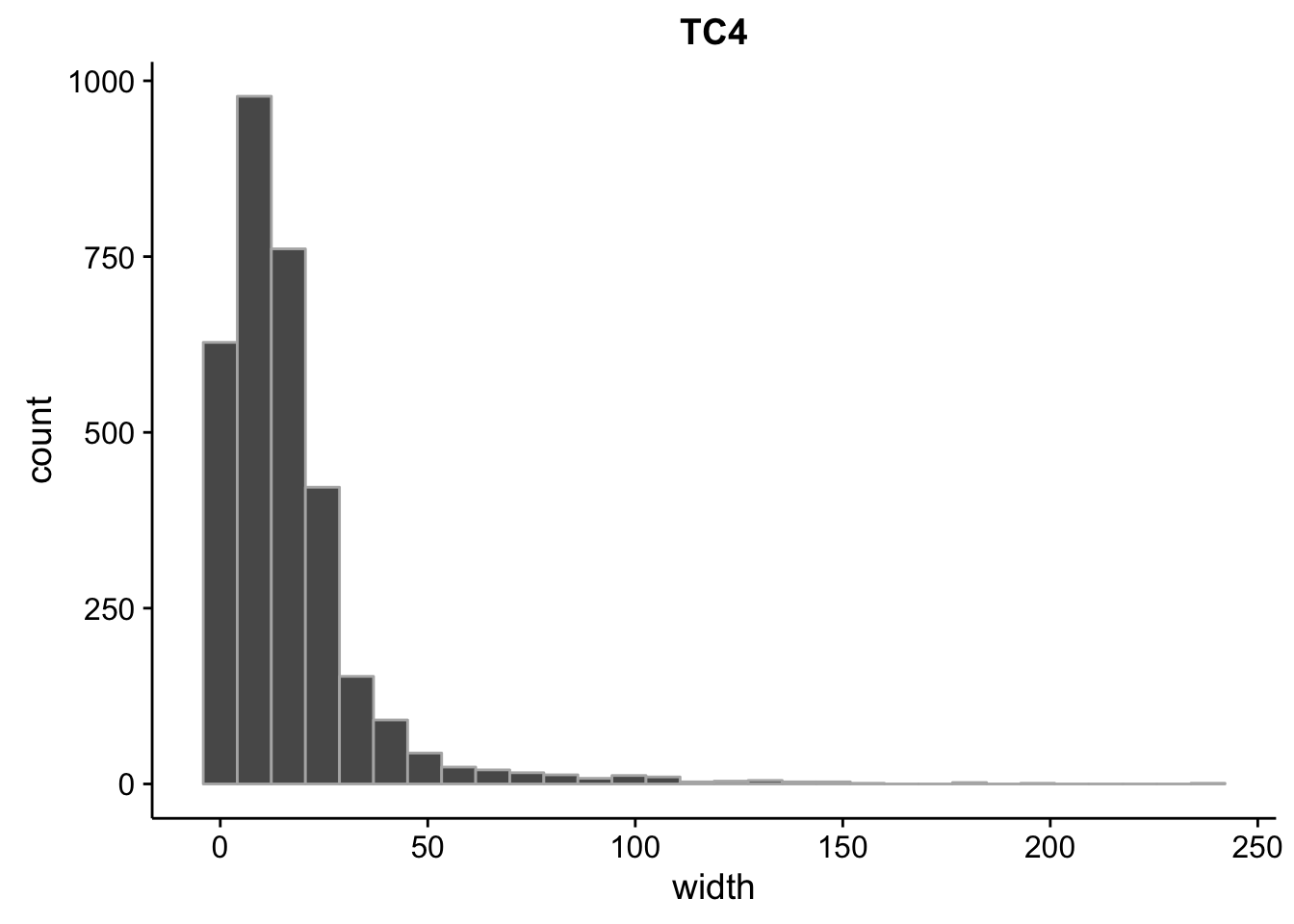

   Min. 1st Qu.  Median    Mean 3rd Qu.    Max. 
   2.00    6.00   13.00   17.85   22.00  230.00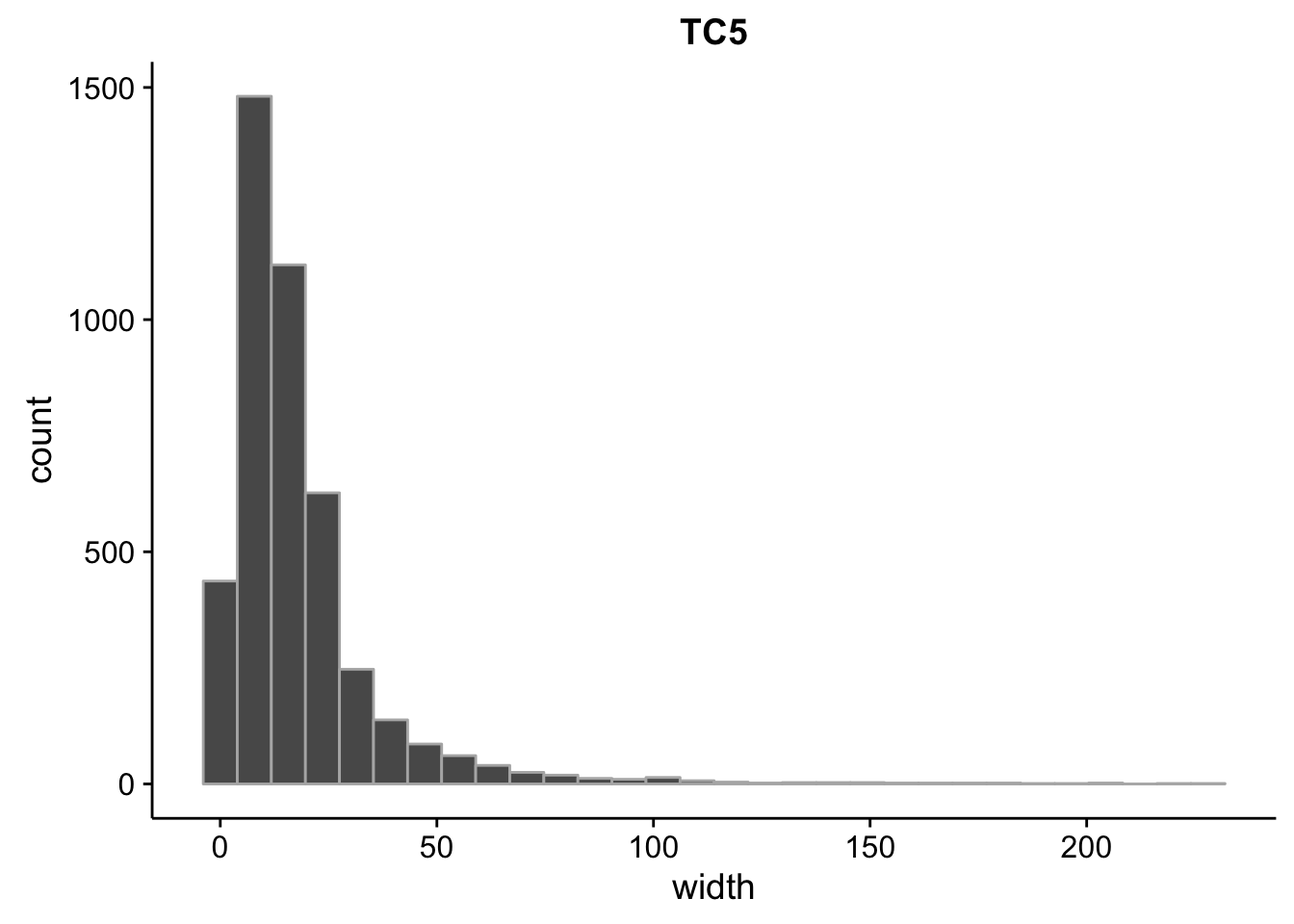

   Min. 1st Qu.  Median    Mean 3rd Qu.    Max. 
   2.00    6.00   12.00   15.84   20.00  238.00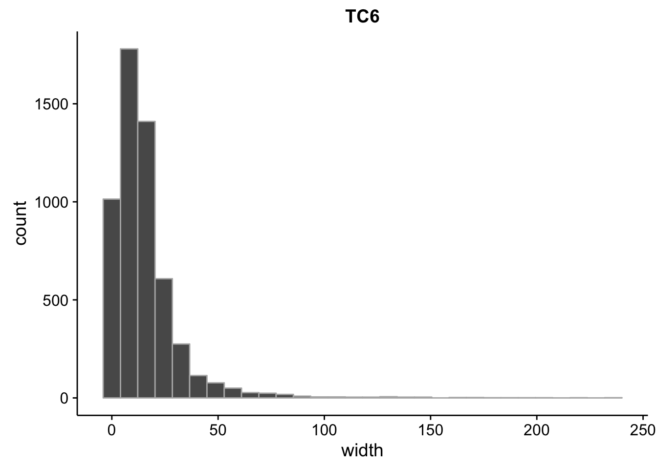

   Min. 1st Qu.  Median    Mean 3rd Qu.    Max. 
   2.00    5.00   12.00   15.51   19.00  267.00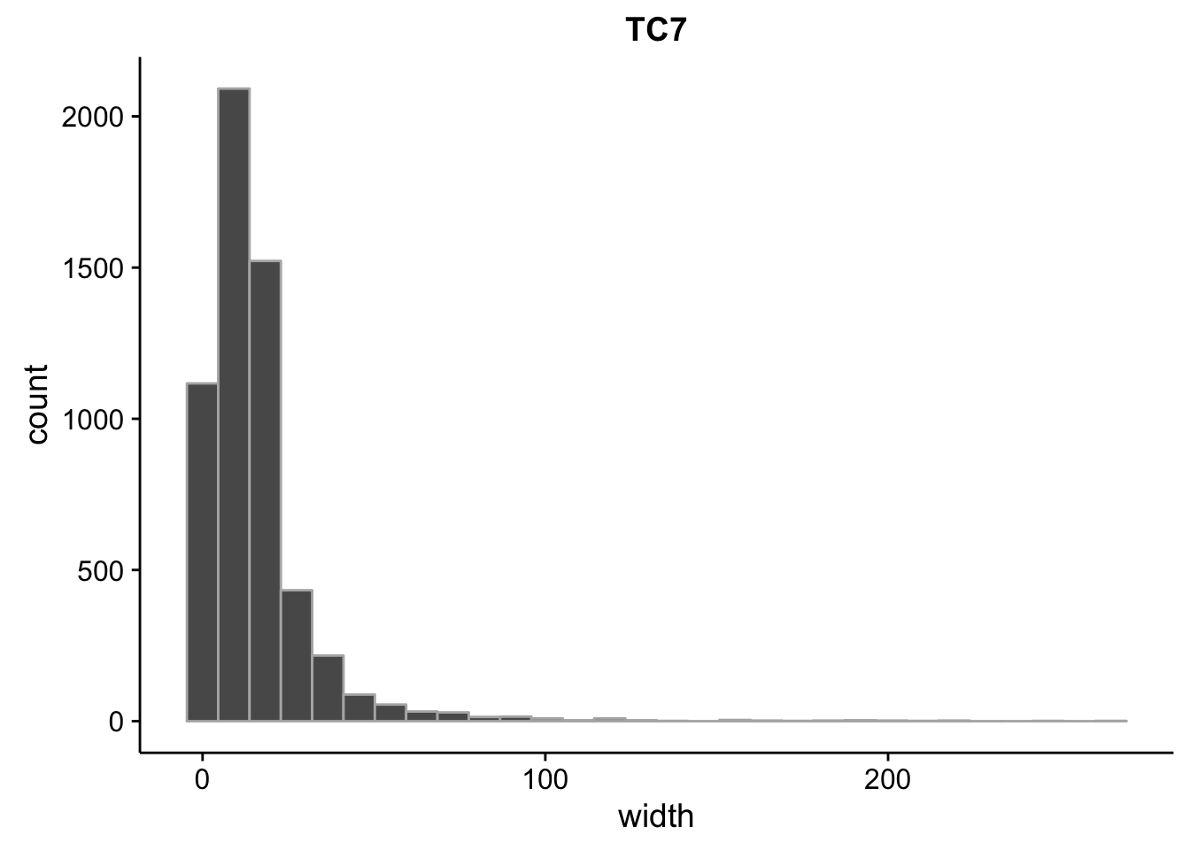

rm(g,s)

What is the coverage of promoter clusters?

We can overlap promoter clusters with tag clusters to calculate the TPM of each and identify the dominant TPM found in each. We can also identify whether there are multiple possible TSSs in each based on how far apart dominant CTSS sites are.

for i in 1 2 3 4 5 6 7; do 
  bedtools intersect -s -wo \
  -a output/ctss_clustering/modified/promoter_clusters.gff \
  -b output/ctss_clustering/modified/tc${i}.gff | \
  awk '{print $1,$2,$3,$4,$5,$6,$7,$8,$18}' > \
  output/ctss_clustering/modified/tc${i}_inter_promoter_clusters.gff
done

Now let’s import those and calculate the total TPM for each:

for (tp in seq(1,7)) {
  f <- paste0("../output/ctss_clustering/modified/tc",tp,"_inter_promoter_clusters.gff")
  assign(x=paste0("pc",tp),value=tibble::as_tibble(rtracklayer::import.gff(f))%>%mutate(tp=tp))
}

Lastly we want to create a set of ranges that identify “orphan” TSSs. If a TSS falls between two converging genes, then don’t annotate it by skipping genes.

# create intergenic regions that appear between convergent genes
genes <- tibble::as_tibble(rtracklayer::import.gff3("../data/annotations/genes_nuclear_3D7_v24.gff"))
convergent <- readr::read_tsv("../output/neighboring_genes/3d7_convergent.tsv")

convergent_ranges <- tibble::tibble(seqnames=character(),start=integer(),end=integer(),strand=character(),left_id=character(),right_id=character())

for (i in 1:nrow(convergent)) {
  left <- genes %>% dplyr::filter(ID %in% convergent$left_gene[i])
  right <- genes %>% dplyr::filter(ID %in% convergent$right_gene[i])
  convergent_ranges <- dplyr::bind_rows(convergent_ranges,
                                        tibble::tibble(seqnames=left$seqnames,
                                        start=left$end,
                                        end=right$start,
                                        strand="*",
                                        left_id=left$ID,
                                        right_id=right$ID))
}

convergent_ranges <- convergent_ranges %>%
  dplyr::filter(end-start>=0) %>%
  GenomicRanges::GRanges()

Annotating clustered tags

Now that we’ve predicted and explored some characteristics of TCs and PCs, we need to annotate each of them. First we need to annotate those that intersect exons and introns. Then remove those from the tag clusters that don’t. Then annotate the intergenic tag clusters and calculate the distances to their annotated features.

tcl <- list(tc1,tc2,tc3,tc4,tc5,tc6,tc7)

for (i in 1:length(tcl)) {
  # one tag cluster sample at a time
  # change to single nucleotide length
  # to ensure proper annotation
  tc <- tcl[[i]] %>%
    tibble::as_tibble() %>%
    dplyr::rename(full_end=end) %>%
    dplyr::mutate(end=start) %>%
    GenomicRanges::GRanges()

  # overlap with known exons
  # bind the columns together
  one <- tibble::as_tibble(tc[tibble::as_tibble(GenomicRanges::findOverlaps(tc,exons.bed))$queryHits])
  two <- tibble::as_tibble(exons.bed[tibble::as_tibble(GenomicRanges::findOverlaps(tc,exons.bed))$subjectHits]) %>%
    dplyr::select(name,anno_start,anno_end)
  assign(paste0("tc",i,"_exons"),value=dplyr::bind_cols(one,two) %>% mutate(tp=i))
  
  # overlap with known introns
  # bind columns together
  one <- tibble::as_tibble(tc[tibble::as_tibble(GenomicRanges::findOverlaps(tc,introns.bed))$queryHits])
  two <- tibble::as_tibble(introns.bed[tibble::as_tibble(GenomicRanges::findOverlaps(tc,introns.bed))$subjectHits]) %>%
    dplyr::select(name,anno_start,anno_end)
  assign(paste0("tc",i,"_introns"),value=dplyr::bind_cols(one,two) %>% mutate(tp=i))
  
  # remove tag clusters that overlap with known genes and fall between convergent genes
  # find which feature in 'subject' the tag cluster precedes
  # bind columns together
  tc <- tc[!1:length(tc) %in% tibble::as_tibble(GenomicRanges::findOverlaps(tc,genes.bed))$queryHits]
  tc <- tc[!1:length(tc) %in% tibble::as_tibble(GenomicRanges::findOverlaps(tc,convergent_ranges))$queryHits]
  one <- tibble::as_tibble(tc[!is.na(GenomicRanges::precede(tc,genes.bed))])
  two <- tibble::as_tibble(genes.bed[na.omit(GenomicRanges::precede(tc,genes.bed))]) %>%
    dplyr::select(name,anno_start,anno_end)
  assign(paste0("tc",i,"_intergenic"),value=dplyr::bind_cols(one,two) %>% mutate(tp=i))
}
# combine into a single table
tc_intergenic <- dplyr::bind_rows(tc1_intergenic,tc2_intergenic,
                                  tc3_intergenic,tc4_intergenic,
                                  tc5_intergenic,tc6_intergenic,
                                  tc7_intergenic) %>%
  dplyr::select(-width,-source,-type,-score,-phase)

# combine into a single table
tc_exons <- dplyr::bind_rows(tc1_exons,tc2_exons,
                                  tc3_exons,tc4_exons,
                                  tc5_exons,tc6_exons,
                                  tc7_exons) %>%
  dplyr::select(-width,-source,-type,-score,-phase)

# combine into a single table
tc_introns <- dplyr::bind_rows(tc1_introns,tc2_introns,
                                  tc3_introns,tc4_introns,
                                  tc5_introns,tc6_introns,
                                  tc7_introns) %>%
  dplyr::select(-width,-source,-type,-score,-phase)

rm(one,two,tc,tcl)

rtracklayer::export.gff3(GenomicRanges::GRanges(tc_intergenic),"../output/ctss_clustering/modified/tag_clusters_annotated_intergenic.gff")
rtracklayer::export.gff3(GenomicRanges::GRanges(tc_exons),"../output/ctss_clustering/modified/tag_clusters_annotated_exons.gff")
rtracklayer::export.gff3(GenomicRanges::GRanges(tc_introns),"../output/ctss_clustering/modified/tag_clusters_annotated_introns.gff")

Now let’s do the same for PCs that have been intersect with TCs as seen above:

pc <- dplyr::bind_rows(pc1,pc2,pc3,pc4,pc5,pc6,pc7) %>%
  dplyr::rename(full_end=end) %>%
  dplyr::mutate(end=start)

# overlap known exons
# bind columns together
one <- pc[tibble::as_tibble(GenomicRanges::findOverlaps(GenomicRanges::GRanges(pc),exons.bed))$queryHits,]
two <- tibble::as_tibble(exons.bed[tibble::as_tibble(GenomicRanges::findOverlaps(GenomicRanges::GRanges(pc),exons.bed))$subjectHits]) %>%
  dplyr::select(name,anno_start,anno_end)
pc_exons <- dplyr::bind_cols(one,two) %>%
  dplyr::select(-width,-source,-type,-score,-phase)
  
# overlap with known introns
# bind columns together
one <- pc[tibble::as_tibble(GenomicRanges::findOverlaps(GenomicRanges::GRanges(pc),introns.bed))$queryHits,]
two <- tibble::as_tibble(introns.bed[tibble::as_tibble(GenomicRanges::findOverlaps(GenomicRanges::GRanges(pc),introns.bed))$subjectHits]) %>%
  dplyr::select(name,anno_start,anno_end)
pc_introns <- dplyr::bind_cols(one,two) %>%
  dplyr::select(-width,-source,-type,-score,-phase)
  
# remove tag clusters that overlap with known genes and fall between convergent genes
# find which feature in 'subject' the tag cluster precedes
# bind columns together
tmp <- pc[!1:length(pc) %in% tibble::as_tibble(GenomicRanges::findOverlaps(GenomicRanges::GRanges(pc),genes.bed))$queryHits,]
tmp <- pc[!1:length(pc) %in% tibble::as_tibble(GenomicRanges::findOverlaps(GenomicRanges::GRanges(pc),convergent_ranges))$queryHits,]
one <- tmp[!is.na(GenomicRanges::precede(GenomicRanges::GRanges(tmp),genes.bed)),]
two <- tibble::as_tibble(genes.bed[na.omit(GenomicRanges::precede(GenomicRanges::GRanges(tmp),genes.bed))]) %>%
  dplyr::select(name,anno_start,anno_end)
pc_intergenic <- dplyr::bind_cols(one,two) %>%
  dplyr::select(-width,-source,-type,-score,-phase)

rm(one,two,tmp)

Before we continue, we should write these to a file:

rtracklayer::export.gff3(GenomicRanges::GRanges(pc_intergenic),"../output/ctss_clustering/modified/promoter_clusters_annotated_intergenic.gff")
rtracklayer::export.gff3(GenomicRanges::GRanges(pc_exons),"../output/ctss_clustering/modified/promoter_clusters_annotated_exons.gff")
rtracklayer::export.gff3(GenomicRanges::GRanges(pc_introns),"../output/ctss_clustering/modified/promoter_clusters_annotated_introns.gff")

Finally, we can look at the distribution of annotations. Which genes have many TCs? Many PCs? And how many do we see on average? To do this we need to first remove duplicates from our list and then filter by expression levels.

Here we will divide the tag clusters into individual time points:

tc_intergenic %>% 
  dplyr::group_by(seqnames,start,end,name,tp) %>% 
  dplyr::filter(as.numeric(tpm.dominant_ctss) >= 5) %>%
  dplyr::group_by(name,tp) %>% 
  dplyr::summarise(n=n()) %>% 
  dplyr::group_by(tp) %>%
  dplyr::summarise(mean=mean(n),median=median(n),min=min(n),max=max(n))

# A tibble: 7 × 5
     tp     mean median   min   max
  <int>    <dbl>  <dbl> <int> <int>
1     1 1.589219      1     1     9
2     2 1.651477      1     1     9
3     3 1.455992      1     1     9
4     4 1.423968      1     1     8
5     5 1.450718      1     1     8
6     6 1.483022      1     1     7
7     7 1.521053      1     1    10

tc_intergenic %>% 
  dplyr::group_by(seqnames,start,end,name,tp) %>% 
  dplyr::filter(as.numeric(tpm.dominant_ctss) >= 5) %>%
  dplyr::group_by(name,tp) %>% 
  dplyr::summarise(n=n()) %>% 
  ggplot(aes(x=n)) + 
  geom_histogram(color="grey70") +
  facet_grid(~tp)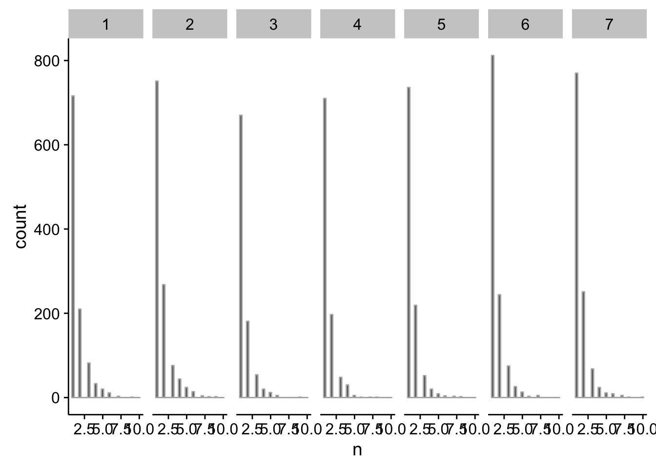

And here we’ll look at promoter clusters all together:

pc_intergenic %>% 
  dplyr::group_by(seqnames,start,end,name) %>% 
  dplyr::summarise(tpm=sum(as.numeric(tpm))) %>% 
  dplyr::filter(tpm >= 5) %>%
  dplyr::group_by(name) %>% 
  dplyr::summarise(n=n()) %>% 
  summary()

     name                 n         
 Length:3324        Min.   : 1.000  
 Class :character   1st Qu.: 1.000  
 Mode  :character   Median : 1.000  
                    Mean   : 1.521  
                    3rd Qu.: 2.000  
                    Max.   :11.000

pc_intergenic %>% 
  dplyr::group_by(seqnames,start,end,name) %>% 
  dplyr::summarise(tpm=sum(as.numeric(tpm))) %>% 
  dplyr::filter(tpm >= 5) %>%
  dplyr::group_by(name) %>% 
  dplyr::summarise(n=n()) %>% 
  ggplot(aes(x=n)) + 
  geom_histogram(color="grey70")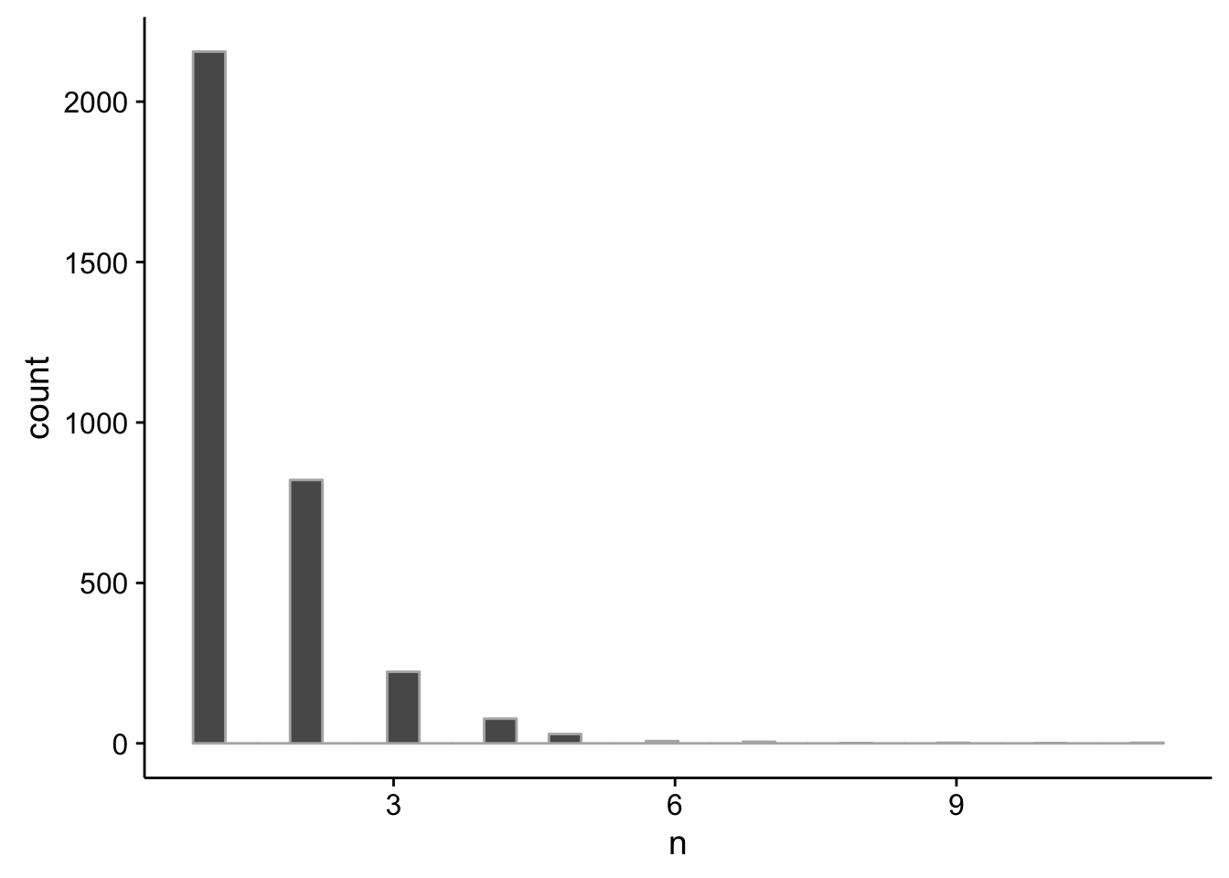

Annotating ‘shifting promoters’

CAGEr can also detect ‘shifting promoters’. These are promoters where we see significant changes in the dominant CTSS within a single promoter.

files <- list.files(path="../output/ctss_clustering/modified",pattern="shifting_promoters",full.names=TRUE)

shifting <- tibble::tibble(
  consensus.cluster=integer(),
  chr=character(),
  start=integer(),
  end=integer(),
  strand=character(),
  shifting.score=double(),
  groupX.pos=integer(),
  groupY.pos=integer(),
  groupX.tpm=double(),
  groupY.tpm=double(),
  pvalue.KS=double(),
  fdr.KS=double())

for (file in files) {
  shifting <- dplyr::bind_rows(shifting,read_tsv(file,col_names=TRUE))
}

Not every detected shift is spatial so we can calculate the degree of spatial shifting and filter only those that shift significantly:

annotated_shifting <- shifting %>% 
  dplyr::mutate(shift=abs(groupX.pos-groupY.pos)) %>% 
  dplyr::filter(shift>=100) %>% 
  dplyr::distinct(chr,start,end,strand,groupX.pos,groupY.pos) %>% 
  dplyr::arrange(chr,start) %>%
  dplyr::inner_join(pc_intergenic, by = c("chr"="seqnames","start","strand")) %>%
  dplyr::distinct(chr,start,end.x,name,groupX.pos,groupY.pos) %>%
  dplyr::rename(end=end.x)

Now we can write that to output:

write_tsv(x=annotated_shifting,path="../output/ctss_clustering/modified/annotated_shifting.tsv")

Session Information

sessionInfo()

R version 3.3.2 (2016-10-31)
Platform: x86_64-apple-darwin15.6.0 (64-bit)
Running under: OS X El Capitan 10.11.6

locale:
[1] en_US.UTF-8/en_US.UTF-8/en_US.UTF-8/C/en_US.UTF-8/en_US.UTF-8

attached base packages:
[1] stats     graphics  grDevices utils     datasets  methods   base     

other attached packages:
 [1] scales_0.4.1    cowplot_0.7.0   magrittr_1.5    stringr_1.2.0  
 [5] dplyr_0.5.0     purrr_0.2.2     readr_1.0.0     tidyr_0.6.1    
 [9] tibble_1.2      ggplot2_2.2.1   tidyverse_1.1.1

loaded via a namespace (and not attached):
 [1] SummarizedExperiment_1.4.0 reshape2_1.4.2            
 [3] haven_1.0.0                lattice_0.20-34           
 [5] colorspace_1.3-2           htmltools_0.3.5           
 [7] stats4_3.3.2               rtracklayer_1.34.2        
 [9] yaml_2.1.14                XML_3.98-1.5              
[11] foreign_0.8-67             DBI_0.5-1                 
[13] BiocParallel_1.8.1         BiocGenerics_0.20.0       
[15] modelr_0.1.0               readxl_0.1.1              
[17] plyr_1.8.4                 zlibbioc_1.20.0           
[19] Biostrings_2.42.1          munsell_0.4.3             
[21] gtable_0.2.0               workflowr_0.3.0           
[23] rvest_0.3.2                psych_1.6.12              
[25] evaluate_0.10              labeling_0.3              
[27] Biobase_2.34.0             knitr_1.15.1              
[29] forcats_0.2.0              IRanges_2.8.1             
[31] GenomeInfoDb_1.10.3        parallel_3.3.2            
[33] broom_0.4.2                Rcpp_0.12.9               
[35] backports_1.0.5            S4Vectors_0.12.1          
[37] jsonlite_1.3               XVector_0.14.0            
[39] Rsamtools_1.26.1           mnormt_1.5-5              
[41] hms_0.3                    digest_0.6.12             
[43] stringi_1.1.2              GenomicRanges_1.26.3      
[45] grid_3.3.2                 rprojroot_1.2             
[47] tools_3.3.2                bitops_1.0-6              
[49] lazyeval_0.2.0             RCurl_1.95-4.8            
[51] Matrix_1.2-8               xml2_1.1.1                
[53] lubridate_1.6.0            assertthat_0.1            
[55] rmarkdown_1.3              httr_1.2.1                
[57] R6_2.2.0                   GenomicAlignments_1.10.0  
[59] nlme_3.1-131               git2r_0.18.0

This R Markdown site was created with workflowr